Chapter Notes- Unit 1: Measures of Central Tendency


Unit Overview
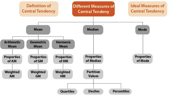
Definition of Central Tendency
In various cases, such as the distributions of height, weight, marks, profit, and wages, it has been observed that the class frequency starts off low, gradually increases to a maximum around the central part of the distribution, and then steadily decreases towards the end. Central tendency refers to the tendency of a given set of observations to cluster around a single central or middle value. The single value that represents the given set of observations is called a measure of central tendency, location, or average. This means that a large amount of data can be condensed into a single representative value.
Computing a measure of central tendency is crucial in many areas. For example, a company is recognized by its high average profit, and an educational institution is judged based on the average marks obtained by its students. Central tendency also provides a basis for comparing different distributions. There are different measures of central tendency, including:
(i) Mean
- Arithmetic Mean (AM)
- Geometric Mean (GM)
- Harmonic Mean (HM)
(ii) Median (Me)
(iii) Mode (Mo)
Criteria for an Ideal Measure of Central Tendency
Following are the criteria for an ideal measure of central tendency:
(i) It should be properly and unambiguously defined.
(ii) It should be easy to comprehend.
(iii) It should be simple to compute.
(iv) It should be based on all the observations.
(v) It should have certain desirable mathematical properties.
(vi) It should be least affected by the presence of extreme observations.
Arithmatic Mean
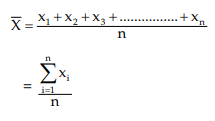
- The Arithmetic Mean (AM) is calculated by taking the sum of all observations and dividing it by the total number of observations.
- For a variable x that has n values, which can be represented as x1, x2, x3, ..., xn, the formula for the AM can be expressed as:
- AM = (x1 + x2 + x3 + ... + xn) / n
- This means you add up each value of x and then divide that total by n, the number of values.
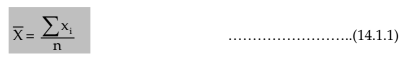
In case of a simple frequency distribution relating to an attribute, we have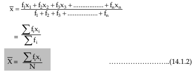
assuming the observation xi occurs fi times, i = 1,2,3,........n and N = ∑f i. In case of grouped frequency distribution also we may use formula (14.1.2) with xi as the mid value of the i-th class interval, on the assumption that all the values belonging to the i-th class interval are equal to xi.
However, in most cases, if the classification is uniform, we consider the following formula for the computation of AM from grouped frequency distribution:

Where, 
A = Assumed Mean
C = Class Length
ILLUSTRATIONS:
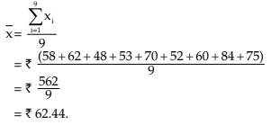
Example 14.1.1: Following are the daily wages in Rupees of a sample of 9 workers: 58, 62, 48, 53, 70, 52, 60, 84, 75. Compute the mean wage.
Solution: Let x denote the daily wage in rupees.
SThen as given, x1 = 58, x2 = 62, x3 = 48, x4 = 53, x5 = 70 , x6 = 52, x7 = 60, x8 = 84 and x9 = 75.
Applying (14.1.1) the mean wage is given by,
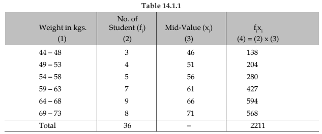
Example 14.1.2: Compute the mean weight of a group of BBA students of St. Xavier's College from the following data:
Solution:Computation of mean weight of 36 BBA students
Applying (14.1.2), we get the average weight as
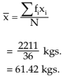
Example 14.1.3: Find the AM for the following distribution:

Solution: We apply formula (14.1.3) since the amount of computation involved in finding the AM is much more compared to Example 14.1.2. Any mid value can be taken as A. However, usually A is taken as the middle most mid-value for an odd number of class intervals and any one of the two middle most mid-values for an even number of class intervals. The class length is taken as C.
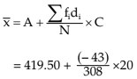
The required AM is given by
= 419.50 - 2.79
= 416.71
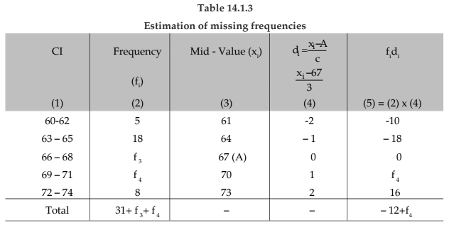
Example 14.1.4: Given that the mean height of a group of students is 67.45 inches. Find the missing frequencies for the following incomplete distribution of height of 100 students.

Solution: Let x denote the height and f3 and f4 as the two missing frequencies.
As given, we have
Thus, the missing frequencies would be 42 and 27.

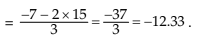
Properties of AM
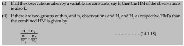
(i) If all the observations assumed by a variable are constants, say k, then the AM is also k. For example, if the height of every student in a group of 10 students is 170 cm, then the mean height is, of course, 170 cm.(ii) 
- For example, if a variable x has five values: 58, 63, 37, 45, and 29, then the average
 is 46.4.
 - The differences between each value and the average (AM) are calculated as follows:
- From 58, the difference is 11.60.
- From 63, the difference is 16.60.
- From 37, the difference is -9.40.
- From 45, the difference is -1.40.
- From 29, the difference is -17.40.
- The sum of these differences is:
- 11.60 + 16.60 + -9.40 + -1.40 + -17.40 = 0.
(iii) 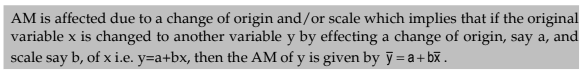
For example, if it is known that two variables x and y are related by 2x+3y+7=0 and  , then the AM of y is given by
(iv) If there are two groups containing n1 and n2 observations  as the respective arithmetic means, then the combined AM is given by
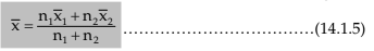
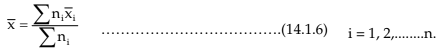
This property could be extended to k>2 groups and we may write
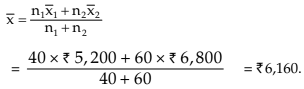
Example 14.1.5: The mean salary for a group of 40 female workers is ₹5,200 per month and that for a group of 60 male workers is ₹ 6800 per month. What is the combined mean salary?
Solution: As given
hence, the combined mean salary per month is
Median - Partition Values
Compared to the arithmetic mean (AM), the median is a positional average. This means that the value of the median depends on the arrangement of the data points in the set.The median can be defined as the middle value when the data points are sorted in either ascending or descending order.
For example, consider the marks of 7 students: 72, 85, 56, 80, 65, 52, and 68.
To find the median mark, we first arrange the marks in ascending order: 52, 56, 65, 68, 72, 80, 85.
Here, the 4th term (68) is the middle value, so the median mark is 68.
In another example, let's look at the wages of 8 workers, given in rupees: 56, 82, 96, 120, 110, 82, 106, and 100.
- Arranging these wages in ascending order gives us: 56, 82, 82, 96, 100, 106, 110, 120.
- In this case, there are two middle values: 96 and 100.
- Any value between 96 and 100 could be considered a median wage. However, to make it unique, we take the arithmetic mean of these two middle values when the number of observations is even.
Thus, the median wage in this example, would be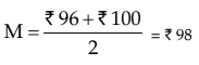 In case of a grouped frequency distribution, we find median from the cumulative frequency distribution of the variable under consideration. We may consider the following formula, which can be derived from the basic definition of median.
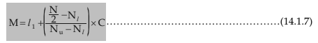
Where,
l1 = lower class boundary of the median class i.e. the class containing median.
N = total frequency.
Nl = less than cumulative frequency corresponding to l1. (Pre median class)
Nu = less than cumulative frequency corresponding to l2. (Post median class)
l2 being the upper class boundary of the median class.
C = l2 - l1 = length of the median class.
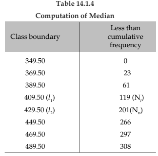
Example 14.1.6: Compute the median for the distribution as given in Example 14.1.3.
Solution: First, we find the cumulative frequency distribution which is exhibited in Table 14.1.4.
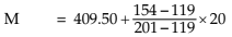
We find, from the Table 14.1.4, N/2 = 308/2 lies between the two cumulative frequencies 119 and 201 i.e. 119 < 154 < 201 . Thus, we have Nl = 119, Nu = 201 l1 = 409.50 and l2 = 429.50. Hence C = 429.50 - 409.50 =20.
Substituting these values in (14.1.7), we get,
= 409.50+8.54 = 418.04.
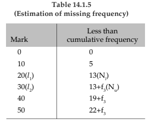
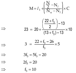
Example 14.1.7: Find the missing frequency from the following data, given that the median mark is 23.

Solution: Let us denote the missing frequency by f3. Table 14.1.5 shows the relevant computation.
Going through the mark column, we find that 20<23<30. Hence l1 = 20, l2 =30 and accordingly Nl = 13, Nu =13 + f3. Also the total frequency i.e. N is 22 + f3. Thus,
So, the missing frequency is 10.
Properties of median
We cannot treat median mathematically, the way we can do with arithmetic mean. We consider below two important features of median.
(i) If x and y are two variables, to be related by y=a + bx for any two constants a and b, then the median of y is given by yme = a + bxme
For example, if the relationship between x and y is given by 2x - 5y = 10 and if x me i.e. the median of x is known to be 16.
Then 2x - 5y = 10
⇒ y = -2 + 0.40x
⇒ yme = -2 + 0.40 x me
⇒ yme = -2 + 0.40 × 16
⇒ yme = 4.40.
(ii) For a set of observations, the sum of absolute deviations is minimum when the deviations are taken from the median. This property states that ∑|xi - A| is minimum if we choose A as the median.
Partition Values or Quartiles or Fractiles
- These are values that split a set of observations into equal parts.
- When dividing a set of observations into two equal parts, we look at the median.
Quartilessplit the observations into four equal parts. There are three quartiles:
- Q1 - the first quartile or lower quartile, where one fourth of the data is less than or equal to this value, and three fourths are greater.
- Q2 - the second quartile, also known as the median.
- Q3 - the third quartile or upper quartile, where three fourths of the data is less than or equal to this value, and one fourth is greater.
Deciles divide the observations into ten equal parts, with nine deciles identified as D1, D2, D3, ..., D9.
- D1 - the first decile, where one tenth of the observations are less than or equal to this value, and nine tenths are greater when arranged in order.
Percentiles, or centiles, divide the observations into 100 equal parts, with the points of division labeled P1, P2, ..., P99.
- P1 - the first percentile, where one hundredth of the observations are less than or equal to this value, and ninety-nine hundredths are greater when arranged in order.
- For ungrouped data, the pth quartile can be found using the formula (n + 1) * p, where nis the total number of observations:
- For Q1, Q2, and Q3, p equals 1/4, 2/4, and 3/4 respectively.
- For D1 to D9, p equals 1/10, 2/10, ..., 9/10.
- For P1 to P99, p equals 1/100, 2/100, ..., 99/100.
In case of a grouped frequency distribution, we consider the following formula for the computation of quartiles.
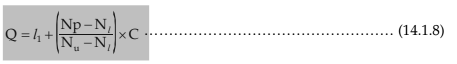
The symbols, except p, have their usual interpretation which we have already discussed while computing median and just like the unclassified data, we assign different values to p depending on the quartile.
Another way to find quartiles for a grouped frequency distribution is to draw the ogive (less than type) for the given distribution. In order to find a particular quartile, we draw a line parallel to the horizontal axis through the point Np. We draw perpendicular from the point of intersection of this parallel line and the ogive. The x-value of this perpendicular line gives us the value of the quartile under discussion.
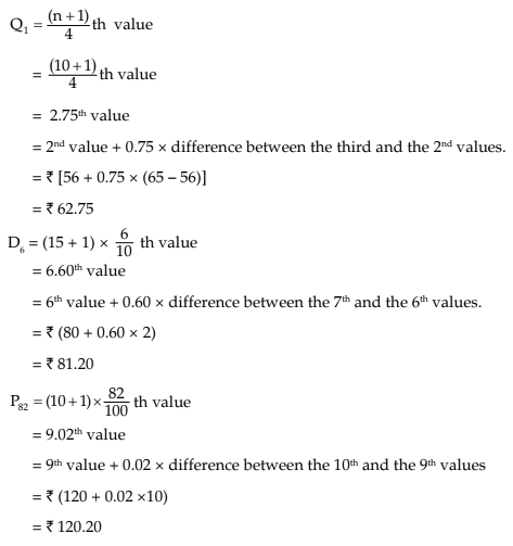
Example 14.1.8: Following are the wages of the labourers: ₹ 82, ₹ 56, ₹ 90, ₹ 50, ₹ 120, ₹ 75, ₹ 75, ₹ 80, ₹ 130, ₹ 65. Find Q1, D6 and P82.
Solution: Arranging the wages in an ascending order, we get ₹ 50, ₹ 56, ₹ 65, ₹ 75, ₹ 75, ₹ 80, ₹ 82, ₹ 90, ₹ 120, ₹ 130.
Hence, we have
Next, let us consider one problem relating to the grouped frequency distribution.
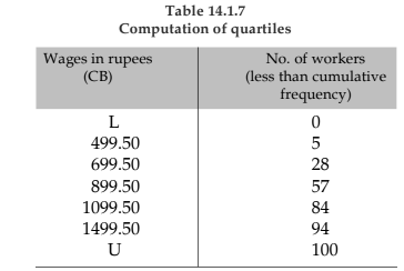
Example 14.1.9: Following distribution relates to the distribution of monthly wages of 100 workers.

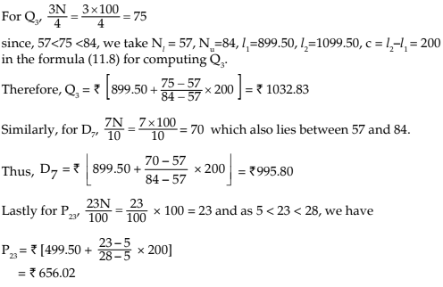
Compute Q3 , D7 and P23 .
Solution: This is a typical example of an open end unequal classification as we find the lower class limit of the first class interval and the upper class limit of the last class interval are not stated, and theoretically, they can assume any value between 0 and 500 and 1500 to any number respectively. The ideal measure of the central tendency in such a situation is median as the median or second quartile is based on the fifty percent central values. Denoting the first LCB and the last UCB by the L and U respectively, we construct the following cumulative frequency distribution:
Mode
- The mode is the value that appears the most frequently in a set of observations.
- In other words, the mode is the value around which most observations are concentrated, making it the most common value.
- For example, in the list of numbers 5, 3, 8, 9, 5, and 6, the mode is 5 because it appears two times, while all other numbers only appear once.
- The mode can sometimes have more than one value. If a set has multiple modes, it is called a multi-modal distribution.
- If there are exactly two modes, it is referred to as a bi-modal distribution.
It is important to note that a mode may not always exist. For instance, if we look at the marks of five students: 50, 60, 35, 40, and 56, there is no mode because each mark occurs only once.
We may consider the following formula for computing mode from a grouped frequency distribution:
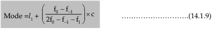
where,
l1 = LCB of the modal class. i.e. the class containing mode.
f0 = frequency of the modal class
f-1 = frequency of the pre-modal class
f1 = frequency of the post modal class
C = class length of the modal class
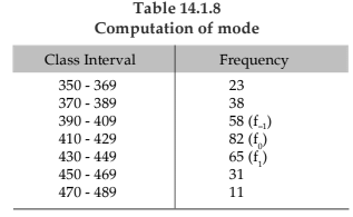
Example 14.1.10: Compute mode for the distribution as described in Example. 14.1.3
Solution: The frequency distribution is shown below:
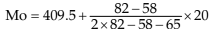
Going through the frequency column, we note that the highest frequency i.e. f0 is 82. Hence, f-1 = 58 and f1 = 65. Also the modal class i.e. the class against the highest frequency is 410 - 429.
Thus l1 = LCB = 409.50 and c = 429.50 - 409.50 = 20
Hence, applying formulas (11.9), we get
= 421.21 which belongs to the modal class. (410 - 429)
When it is difficult to compute mode from a grouped frequency distribution, we may consider the following empirical relationship between mean, median and mode:
Mean - Mode = 3(Mean - Median) .........................(14.1.9A)
or Mode = 3 Median - 2 Mean(14.1.9A) holds for a moderately skewed distribution.
We also note that if y = a + bx, then ymo =a + bxmo ...........................................(14.1.10)
Example 14.11: For a moderately skewed distribution of marks in statistics for a group of 200 students, the mean mark and median mark were found to be 55.60 and 52.40. What is the modal mark?
Solution: Since in this case, mean = 55.60 and median = 52.40, applying (11.9A), we get the modal mark as
Mode = 3 × Median - 2 × Mean
= 3 × 52.40 - 2 × 55.60
= 46.
Example 14.1.12: If y = 2 + 1.50x and mode of x is 15, what is the mode of y?
Solution:
By virtue of (11.10), we have
ymo = 2 + 1.50 × 15
= 24.50.
For a given set of n positive observations, the geometric mean is defined as the n-th root of the product of the observations. Thus if a variable x assumes n values x1, x2, x3,..........., x n, all the values being positive, then the GM of x is given by
G= (x1 × x2 × x3 ........... × xn)1/n ............................................. (14.1.11)
For a grouped frequency distribution, the GM is given by
G= (x1 f1 × x2 f2 × x 3 f3 ................. × xn fn )1/N ............................................. (14.1.12)
Where N = ∑f i
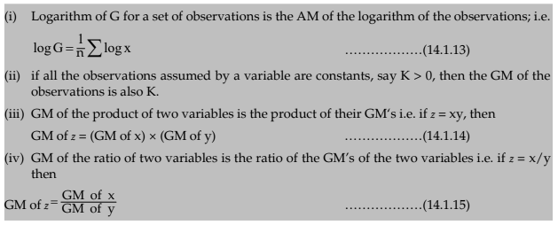
In connection with GM, we may note the following properties :
Example 14.1.13: Find the GM of 3, 6 and 12.
Solution: As given x1 = 3, x2 = 6, x3 = 12 and n = 3.
Applying (14.1.11), we have G = (3 × 6 × 12)1/3 = (63)1/3 = 6.
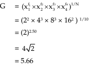
Example 14.1.14: Find the GM for the following distribution:
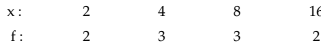
Solution: According to (14.1.12), the GM is given by
Harmonic Mean
The harmonic mean (HM) of a set of non-zero observations is calculated as follows:Given a variable x with n non-zero values: x1, x2, x3, ..., xn, the formula for the harmonic mean is:
HM = n / (1/x1 + 1/x2 + 1/x3 + ... + 1/xn)
Alternatively, it can be expressed as:
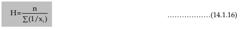
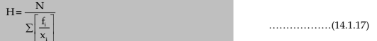
HM = n / Σ(1/xi) where Σ denotes the sum over all observations.
For a grouped frequency distribution, we have
Properties of HM
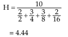
Example 14.15: Find the HM for 4, 6 and 10.
Solution: Applying (14.1.16), we have
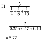
Example 14.1.16: Find the HM for the following data:
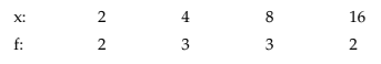
Solution: Using (14.1.17), we get
Relation between AM, GM, and HM
For any set of positive observations, we have the following inequality:
AM ≥ GM ≥ HM .............. (14.1.19)
The equality sign occurs, as we have already seen, when all the observations are equal.
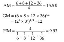
Example 14.1.17: compute AM, GM, and HM for the numbers 6, 8, 12, 36.
Solution: In accordance with the definition, we have
The computed values of AM, GM, and HM establish (14.1.19).
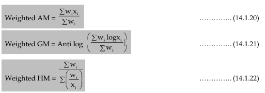
Weighted average
When the observations under consideration have a hierarchical order of importance, we take recourse to computing weighted average, which could be either weighted AM or weighted GM or weighted HM.
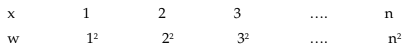
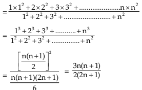
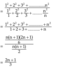
Example 14.1.18: Find the weighted AM and weighted HM of first n natural numbers, the weights being equal to the squares of the corresponding numbers.
Solution: As given,
Weighted
Weighted


A General review of the different measures of central tendency
- In reviewing the various measures of central tendency, it's important to assess their relative advantages and disadvantages based on the criteria for an ideal measure, as previously discussed. The Arithmetic Mean (AM) is generally considered the best measure because it is clearly defined, incorporates all data points, is easy to understand, simple to calculate, and possesses desirable mathematical properties. The mean serves as a stable and reliable average. However, a significant limitation of the AM is its susceptibility to sampling fluctuations. Additionally, in the context of frequency distributions, the mean is not suitable for open-ended classifications.
- The Median also has a clear definition and is straightforward to compute, similar to the AM. However, it does not consider all data points and lacks the ability for extensive mathematical analysis. On the plus side, the median is less influenced by sampling fluctuations and is particularly useful for open-ended classifications.
- One of the main drawbacks of the Arithmetic Mean is its sensitivity to extreme values. While it is commonly believed that the mean is less affected by sampling fluctuations, the median actually experiences more variation from these fluctuations compared to the AM.
- Despite being a popular measure of central tendency, the Mode can sometimes be undefined. Unlike the mean, the mode lacks mathematical properties and is also influenced by sampling fluctuations.
- Geometric Mean (GM) and Harmonic Mean (HM) share some mathematical properties with the AM. They are well-defined and utilize all observations. However, both GM and HM are more complex to understand and calculate, limiting their practical applications to specific scenarios such as average rates and ratios.
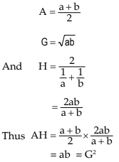
Example 14.1.19: Given two positive numbers a and b, prove that AH = G2. Does the result hold for any set of observations?
Solution: For two positive numbers a and b, we have,
This result holds for only two positive observations and not for any set of observations.
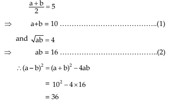
Example 14.1.20: The AM and GM for two observations are 5 and 4 respectively. Find the two observations.
Solution: If a and b are two positive observations then as given
⇒ a - b = 6 (ignoring the negative sign)............................(3)
Adding (1) and (3) We get,
2a = 16
⇒ a= 8
From (1), we get b = 10 - a = 2
Thus, the two observations are 8 and 2.
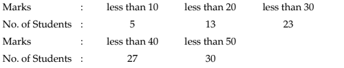
Example 14.1.21: Find the mean and median from the following data:
Also compute the mode using the approximate relationship between mean, median and mode.
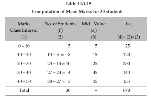
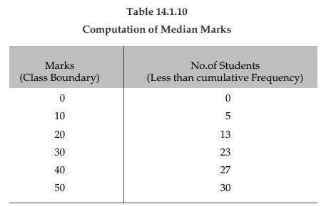
Solution: What we are given in this problem is less than cumulative frequency distribution. We need to convert this cumulative frequency distribution to the corresponding frequency distribution and thereby compute the mean and median.
Hence the mean mark is given by
= 670 / 30
= 22.33
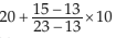
Since lies between 13 and 23, we have l1 = 20, Nl = 13, Nu= 23 and C = l2 - l1 = 30 - 20 = 10
Thus, Median =Since Mode = 3 Median - 2 Mean (approximately), we find that
Mode = 3 x 22 - 2 x 22.33
= 21.34

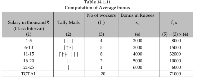
Example 14.1.22: Following are the salaries of 20 workers of a firm expressed in thousand rupees: 5, 17, 12, 23, 7, 15, 4, 18, 10, 6, 15, 9, 8, 13, 12, 2, 12, 3, 15, 14. The firm gave bonus amounting to ₹ 2,000, ₹ 3,000, ₹ 4,000, ₹ 5,000 and ₹ 6,000 to the workers belonging to the salary groups 1,000 - 5,000, 6,000 - 10,000 and so on and lastly 21,000 - 25,000. Find the average bonus paid per employee.
Solution: We first construct frequency distribution of salaries paid to the 20 employees. The average bonus paid per employee is given by
Where xi represents the amount of bonus paid to the ith salary group and f i, the number of employees belonging to that group which would be obtained on the basis of frequency distribution of salaries.
Hence, the average bonus paid per employee
= (₹) 71000 / 20
= (₹) 3550
FAQs on Chapter Notes- Unit 1: Measures of Central Tendency
| 1. What is the definition of central tendency in statistics? |  |
| 2. What are the criteria for an ideal measure of central tendency? | |
| 3. How is the arithmetic mean calculated, and what are its advantages? | |
| 4. What is the difference between median and mode in measures of central tendency? | |
| 5. What is the harmonic mean, and when is it used? | |