Effect of Gain on Root Locus | Control Systems - Electrical Engineering (EE) PDF Download

Introduction

The root locus is a powerful graphical method used in control systems engineering to analyze how the poles of a closed-loop system vary with changes in a system parameter, typically the open-loop gain $\mathrm{<br><span\; style="display:\; none;\; line-height:\; 0;"></span>}K$K. This technique helps engineers predict system stability and performance by plotting the paths of the closed-loop poles as $\mathrm{<br><span\; style="display:\; none;\; line-height:\; 0;"></span>}K$K varies from zero to infinity (or negative infinity in some cases). Understanding the effect of gain on the root locus is crucial, as it directly influences the stability and dynamic behavior of the system. This document, sourced from a Testbook educational capsule, explores the fundamentals of root locus, with a particular emphasis on how gain $\mathrm{<br><span\; style="display:\; none;\; line-height:\; 0;"></span>}K$K affects the pole locations for first-order and second-order systems, along with detailed rules and an example for constructing the root locus.

Root Locus & Its Significance

Usually, the open-loop gain (denoted as $KK$K) is varied. Based on the range of $KK$K, two types of root locus are defined:

• K:0→∞: Root Locus Diagram
• $\mathrm{<br><span\; style="display:\; none;\; line-height:\; 0;"></span>}K:\; 0\; \backslash rightarrow\; -\backslash infty$K:0→−∞: Complementary Root Locus Diagram
• $\mathrm{<br><span\; style="display:\; none;\; line-height:\; 0;"></span>}K:\; -\backslash infty\; \backslash rightarrow\; \backslash infty$K:−∞→∞: Complete Root Locus

The root locus uses the open-loop transfer function to predict closed-loop stability.

Root Locus for First-Order Open-Loop Transfer Function

Consider the transfer function:

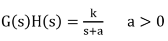
The characteristic equation is:

$q\left(s\right)=1+G\left(s\right)H\left(s\right)=0q(s)\; =\; 1\; +\; G(s)H(s)\; =\; 0$

$\Rightarrow s+a+K=0\backslash Rightarrow\; s\; +\; a\; +\; K\; =\; 0$

$\Rightarrow$s=−(a+K)

Here, the root of the closed-loop equation is a function of $aa$a and the system gain $KK$K. As $KK$K varies, the pole location changes as follows:

The variation of closed loop pole path with the variation of parameter k is given as 

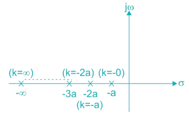
As seen, k is varied from 0 to ∞ the root tends to move left side of the s-plane which means gaining more stability. Thus the system is stable for k ϵ (0, ∞). 

Effect of Gain on Root Locus

The gain $K$K directly affects the position of the closed-loop poles:

• First-Order System: As $K$K increases, the pole shifts further left (e.g., from $-a-a$−a to −∞), enhancing stability by increasing the speed of response.
• Second-Order System: As $\mathrm{<br>}K$K increases, the poles transition from real and distinct (at low $K$K) to real and equal (at $K$= a^2/4 ), and then to complex conjugate pairs (at higher $\mathrm{<br>}K$K), introducing oscillations while remaining stable in the left half-plane.

Number of Lines in Root Locus

In the root locus, lines start from poles and end at zeros. Let the number of zeros be $zz$z and poles be $pp$p:

• If z < p, p - z lines go to infinity (zeros at infinity).
• If p < z, z - p lines come from infinity (poles at infinity).

Rules of Construction of Root Locus

To construct the root locus, the following rules apply:

1. Root locus is symmetrical about the real axis.
2. The number of branches equals the number of finite open-loop poles.
3. Branches start at open-loop poles (K = 0) and end at finite zeros or infinity (K to infinity).
4. A point on the real axis is part of the locus if the total number of poles and zeros to its right is odd.
5. The number of branches going to infinity is p - z.
6. Angle of asymptotes: φa = (2k + 1) × 180° / (p - z), where k = 0, 1, 2, ..., (p - z - 1).
7. Centroid (intersection of asymptotes with real axis): σA = (Summation of real parts of poles - Summation of real parts of zeros) / (p - z).
8. Break-away/break-in points occur where dK/ds = 0.
9. A point on the root locus satisfies: |G(s)H(s)| = 1 and ∠G(s)H(s) = ± (2k + 1) 180°.
10. Intersection with the imaginary axis is found using the Routh-Hurwitz criterion.

Conclusion

The root locus method provides a clear visualization of how the gain K influences the closed-loop pole locations, thereby affecting system stability and response. In first-order systems, increasing K shifts the pole leftward, enhancing stability. In second-order systems, K drives the poles from real to complex, introducing oscillatory behavior while maintaining stability in the left half-plane. By mastering the effect of gain on the root locus and applying construction rules, engineers can design systems with desired performance characteristics. This knowledge is particularly valuable for exams like GATE, where such concepts are frequently tested, emphasizing the practical importance of understanding gain’s role in control system design.