State Space to Transfer Function | Control Systems - Electrical Engineering (EE) PDF Download

Introduction
In control systems engineering, the state-space representation and transfer function are two fundamental approaches to model and analyze dynamic systems. The state-space method provides a time-domain framework, capturing a system’s internal states through a set of first-order differential equations, offering a comprehensive view of its behavior. In contrast, the transfer function approach describes the system in the frequency domain, relating input to output via a ratio of Laplace-transformed polynomials, which is particularly useful for stability and frequency response analysis. Converting from state space to transfer function bridges these two perspectives, enabling engineers to leverage the strengths of both representations—such as detailed state information and simplified input-output relationships—for design, simulation, and control of complex systems.
State Space to Transfer Function
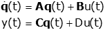
Consider the state space system:
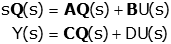
Now, take the Laplace Transform (with zero initial conditions since we are finding a transfer function):
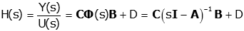
We want to solve for the ratio of Y(s) to U(s), so we need so remove Q(s) from the output equation. We start by solving the state equation for Q(s)
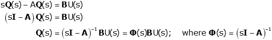
The matrix Φ(s) is called the state transition matrix. Now we put this into the output equation.
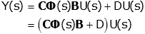 Now we can solve for the transfer function:
Note that although there are many state space representations of a given system, all of those representations will result in the same transfer function (i.e., the transfer function of a system is unique; the state space representation is not).
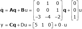
Example: State Space to Transfer Function
Find the transfer function of the system with state space representation
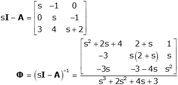
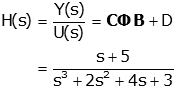
Now we can find the transfer function
To make this task easier, MatLab has a command (ss2tf) for converting from state space to transfer function.
>> % First define state space system
>> A=[0 1 0; 0 0 1; -3 -4 -2];
>> B=[0; 0; 1];
>> C=[5 1 0];
>> [n,d]=ss2tf(A,B,C,D)
n =
0 0 1.0000 5.0000
d =
1.0000 2.0000 4.0000 3.0000
>> mySys_tf=tf(n,d)
Transfer function:
s + 5
----------------------
s^3 + 2 s^2 + 4 s + 3
Properties of the State Transition Matrix
The state transition matrix Φ(s) = (s I - A)^(-1) is central to the conversion process. It represents the system’s dynamic response in the s-domain and has several key properties:- It is a square matrix of size n × n, where n is the number of states.
- Its inverse exists for all s except at the eigenvalues of A (poles of the system).
- The determinant of (s I - A), known as the characteristic polynomial, defines the denominator of the transfer function.
Understanding these properties aids in manual computation and provides insight into system stability, as the poles (roots of det(s I - A) = 0) determine the system’s natural response.
Controllability and Observability in Conversion
The conversion from state space to transfer function assumes the system is controllable and observable:
- Controllability: A system is controllable if the input u(t) can drive all states x(t) to any desired value in finite time. This is checked using the controllability matrix [B AB A^2B ... A^(n-1)B], which must have full rank n.
- Observability: A system is observable if the initial state x(0) can be determined from the output y(t) over time. This is verified using the observability matrix [C; CA; CA^2; ...; CA^(n-1)], which must also have full rank n.
If a system lacks controllability or observability, some modes (poles) may not appear in the transfer function, leading to a reduced-order model—a critical consideration in practical applications.
Effect of Direct Feedthrough Term (D)
The D term in the state space model (y = C x + D u) represents the direct transmission from input to output without involving the states. In the transfer function:
- If D = 0, the transfer function is strictly proper (degree of numerator < degree of denominator).
- If D ≠ 0, the transfer function becomes proper (degree of numerator ≤ degree of denominator), adding a constant term D to G(s).
This affects the system’s high-frequency behavior and steady-state response, making D a key factor in system design and analysis.
Conclusion
The conversion from state space to transfer function is a vital technique in control systems, uniting the detailed, state-based insights of the time domain with the concise, frequency-domain simplicity of transfer functions. This process not only enhances flexibility in system analysis but also facilitates the application of powerful tools like root locus, Bode plots, and controller design, which rely on transfer function models. By mastering this transformation, engineers can seamlessly transition between modeling paradigms, optimizing system performance and stability while addressing practical design challenges, making it an indispensable skill in modern control engineering.
|
53 videos|115 docs|40 tests
|
FAQs on State Space to Transfer Function - Control Systems - Electrical Engineering (EE)
| 1. What is the process to convert a state-space representation to a transfer function? |  |
| 2. What are the properties of the state transition matrix? | |
| 3. What are controllability and observability in the context of state-space systems? | |
| 4. How does the direct feedthrough term (D) affect the transfer function? | |
| 5. Can you provide an example of converting a state-space model to a transfer function? | |


Extra Questions
,MCQs
,Previous Year Questions with Solutions
,mock tests for examination
,Summary
,video lectures
,Free
,practice quizzes
,Viva Questions
,Exam
,Important questions
,Semester Notes
,shortcuts and tricks
,ppt
,State Space to Transfer Function | Control Systems - Electrical Engineering (EE)
,Objective type Questions
,study material
,State Space to Transfer Function | Control Systems - Electrical Engineering (EE)
,State Space to Transfer Function | Control Systems - Electrical Engineering (EE)
,Sample Paper
,past year papers
;


State Space to Transfer Function Free PDF Download
Importance of State Space to Transfer Function
State Space to Transfer Function Notes
State Space to Transfer Function Electrical Engineering (EE) Questions
Study State Space to Transfer Function on the App
|
© EduRev
|
Education Revolution
|


|


