State and Output Feedback


Introduction
This chapter explains how to control systems using feedback in a simple way, focusing on systems that follow straight-line rules and have one control knob. Feedback lets us tweak the system's behavior by setting certain key values (eigenvalues) wherever we want. The "state" is just a set of clues that helps us guess what the system will do next. If we can't directly see the state, we can build a tool called an observer to figure it out using what we know about the system and its inputs and outputs. The controller we end up with matches the system's complexity and has a built-in version of the system itself. Even though we focus on basic systems here, the same ideas work for more complicated ones with lots of controls and results.

Reachability
We begin by disregarding the output measurements and focus on the evolution of the state which is given by
 (5.1)
(5.1)
where x ∈ R.^n , u ∈ R, A is an n × n matrix and B an n × 1 matrix. A fundamental question is if it is possible to find control signals so that any point in the state space can be reached.
First observe that possible equilibria for constant controls are given by
 This means that possible equilibria lies in a one (or possibly higher) dimensional subspace. If the matrix A is invertible this subspace is spanned by A^-1B.
Even if possible equilibria lie in a one dimensional subspace it may still be possible to reach all points in the state space transiently. To explore this we will first give a heuristic argument based on formal calculations with impulse functions. When the initial state is zero the response of the state to a unit step in the input is given by
 (5.2)
(5.2)
The derivative of a unit step function is the impulse function δ(t), which may be regarded as a function which is zero everywhere except at the origin and with the property that
 The response of the system to a impulse function is thus the derivative of (5.2)
Similarly we find that the response to the derivative of a impulse function is
 The input
 thus gives the state
 Hence, right after the initial time t = 0, denoted t = 0+, we have
 The right hand is a linear combination of the columns of the matrix
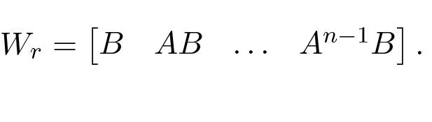 (5.3)To reach an arbitrary point in the state space we thus require that there are n linear independent columns of the matrix Wc. The matrix is called the reachability matrix.
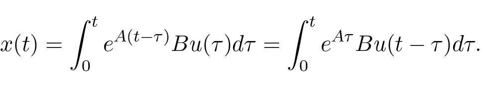
An input consisting of a sum of impulse functions and their derivatives is a very violent signal. To see that an arbitrary point can be reached with smoother signals we can also argue as follow. Assuming that the initial condition is zero, the state of a linear system is given by
 It follows from the theory of matrix functions that

and we find that
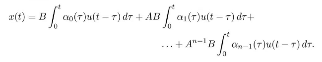
Again we observe that the right hand side is a linear combination of the columns of the reachability matrix Wr given by (5.3).
We illustrate by two examples.
Example 5.1 (Reachability of the Inverted Pendulum). Consider the inverted pendulum example introduced in Example 3.5. The nonlinear equations of motion are given in equation (3.5)
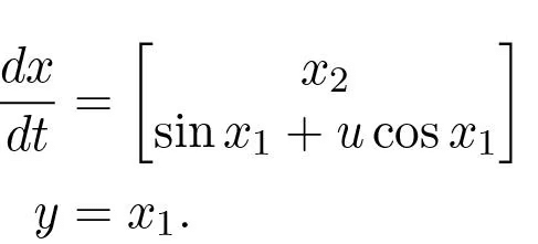 Linearizing this system about x = 0, the linearized model becomes
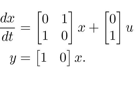 (5.4)
(5.4)
The dynamics matrix and the control matrix are
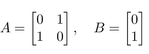 The reachability matrix is
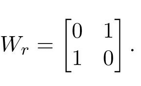 (5.5)This matrix has full rank and we can conclude that the system is reachable. This implies that we can move the system from any initial state to any final state and, in particular, that we can always find an input to bring the system from an initial state to the equilibrium.
Example 5.2 (System in Reachable Canonical Form). Next we will consider a system by in reachable canonical form:
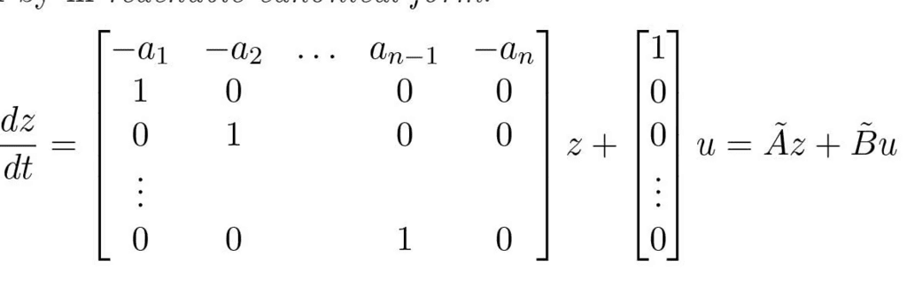 To show that Wr is full rank, we show that the inverse of the reachability matrix exists and is given by
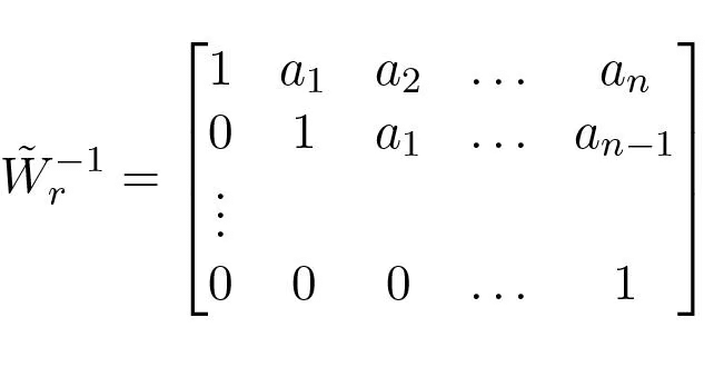 (5.6)To show this we consider the product
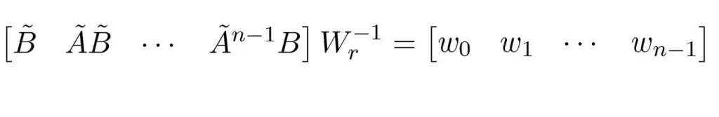 where
where
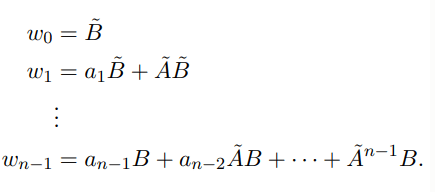
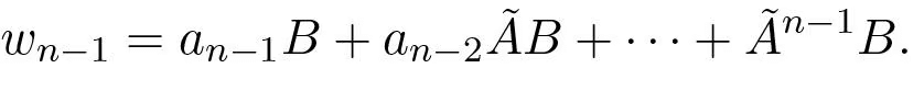 The vectors wk satisfy the relation
and iterating this relation we find that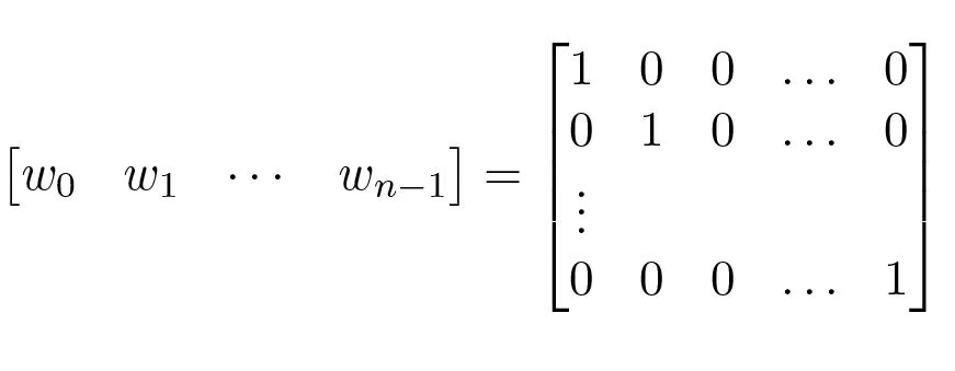 which shows that the matrix (5.6) is indeed the inverse of W˜ r.
Systems That Are Not Reachable
It is useful of have an intuitive understanding of the mechanisms that make a system unreachable. An example of such a system is given in Figure 5.1. The system consists of two identical systems with the same input. The intuition can also be demonstrated analytically. We demonstrate this by a simple example.
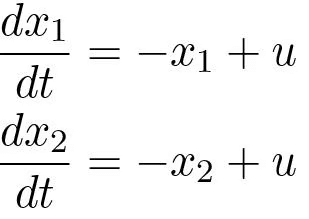
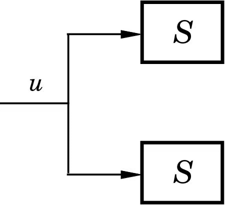 Figure 5.1: A non-reachable system.Example 5.3 (Non-reachable System). Assume that the systems in Figure 5.1 are of first order. The complete system is then described by
 The reachability matrix is
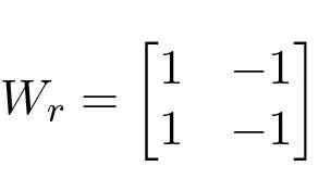
This matrix is singular and the system is not reachable. One implication of this is that if x1 and x2 start with the same value, it is never possible to find an input which causes them to have different values. Similarly, if they start with different values, no input will be able to drive them both to zero.
Coordinate Changes
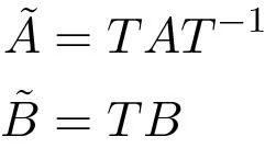
It is interesting to investigate how the reachability matrix transforms when the coordinates are changed. Consider the system in (5.1). Assume that the coordinates are changed to z = T x. As shown in the last chapter, that the dynamics matrix and the control matrix for the transformed system are
The reachability matrix for the transformed system then becomes
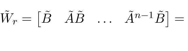 We have
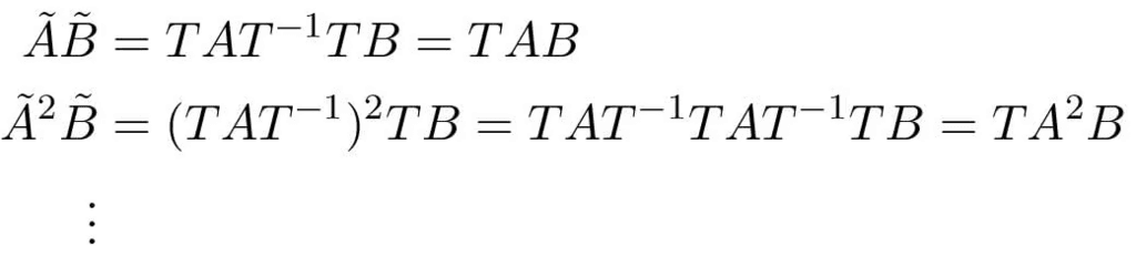
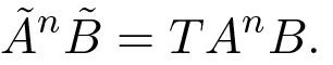
The reachability matrix for the transformed system is thus
 (5.7)This formula is useful for finding the transformation matrix T that converts a system into reachable canonical form (using W˜ r from Example 5.2).
State Feedback
Consider a system described by the linear differential equation
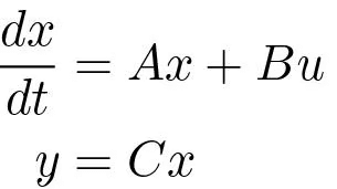 (5.8)The output is the variable that we are interested in controlling. To begin with it is assumed that all components of the state vector are measured. Since the state at time t contains all information necessary to predict the future behavior of the system, the most general time invariant control law is function of the state, i.e.
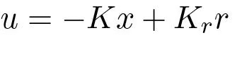
If the feedback is restricted to be a linear, it can be written as
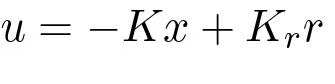 (5.9)where r is the reference value. The negative sign is simply a convention to indicate that negative feedback is the normal situation. The closed loop system obtained when the feedback (5.8) is applied to the system (5.9) is given by
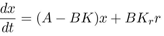 (5.10)
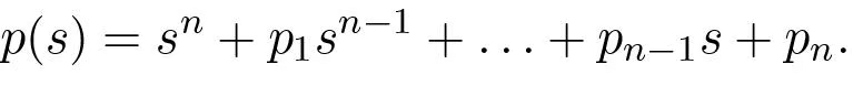
It will be attempted to determine the feedback gain K so that the closed loop system has the characteristic polynomial
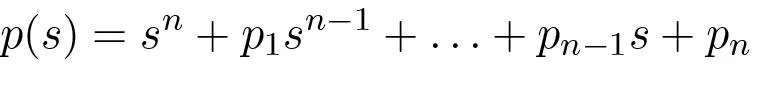 (5.11)This control problem is called the eigenvalue assignment problem or the pole placement problem (we will define "poles" more formally in a later chapter).
Examples
We will start by considering a few examples that give insight into the nature of the problem.
Example 5.4 (The Double Integrator).
The double integrator is described by

Introducing the feedback
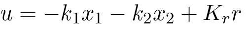
the closed loop system becomes
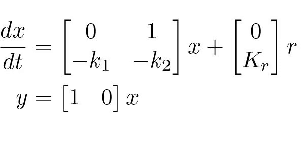
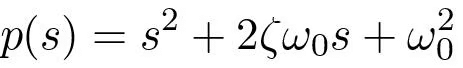
The closed loop system has the characteristic polynomial
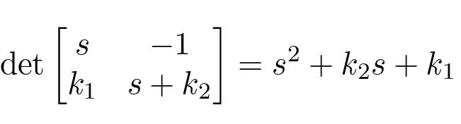 (5.12)
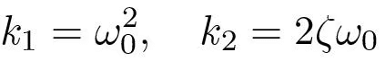
Assume it is desired to have a feedback that gives a closed loop system with the characteristic polynomial
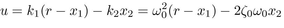
Comparing this with the characteristic polynomial of the closed loop system we find find that the feedback gains should be chosen as
To have unit steady state gain the parameter Kr must be equal to k1 = ω02 . The control law can thus be written as
The General Case
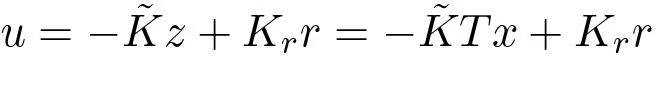
To solve the problem in the general case, we simply change coordinates so that the system is in reachable canonical form. Consider the system (5.8). Change the coordinates by a linear transformation so that the transformed system is in reachable canonical form (5.13). For such a system the feedback is given by (5.14) where the coefficients are given by (5.16). Transforming back to the original coordinates gives the feedback
 It now remains to find the transformation. To do this we observe that the reachability matrices have the property
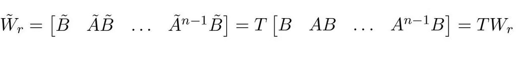
The transformation matrix is thus given by
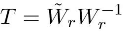 (5.18)
and the feedback gain can be written as
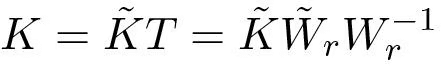 (5.19)
Notice that the matrix W˜ r is given by (5.6). The feedforward gain Kr is given by equation (5.17).
The results obtained can be summarized as follows.
Theorem 5.1 (Pole-placement by State Feedback).
Consider the system given by equation (5.8)
 with one input and one output. If the system is reachable there exits a feedback
 that gives a closed loop system with the characteristic polynomial
 The feedback gain is given by
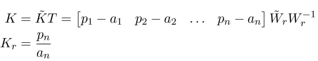
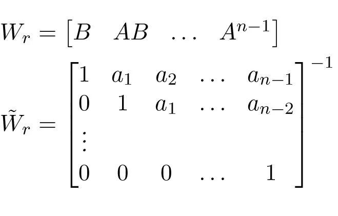
where ai are the coefficients of the characteristic polynomial of the matrix A and the matrices Wr and W˜ r are given by
 Remark 5.1 (A mathematical interpretation). Notice that the eigenvalue placement problem can be formulated abstractly as the following algebraic problem. Given an n × n matrix A and an n × 1 matrix B, find a 1 × n matrix K such that the matrix A - BK has prescribed eigenvalues.
Computing the Feedback Gain
We have thus obtained a solution to the problem and the feedback has been described by a closed form solution.
For simple problems it is easy to solve the problem by the following simple procedure: Introduce the elements ki of K as unknown variables. Compute the characteristic polynomial
Equate coefficients of equal powers of s to the coefficients of the desired characteristic polynomial
This gives a set of equations to figure out the values of ki k_i ki, which can always be solved if the system is observable, like in Example 5.4. For bigger systems, equation (5.19) is easier to use and works for calculations, but with really large systems, it's not as reliable because it involves tricky math with polynomials and big matrix powers. There are better ways to do it numerically, such as using MATLAB's acker or place tools.
Output Feedback
In this section we will consider the same system as in the previous sections, i.e. the nth order system described by
 (5.28)where only the output is measured. As before it will be assumed that u and y are scalars. It is also assumed that the system is reachable and observable. In Section 5.3 we had found a feedback

When all states can be measured, Section 5.4 showed how to build an observer to estimate the state x^ using inputs and outputs. Here, we'll mix these ideas to create a feedback that sets the desired closed-loop eigenvalues for systems where only outputs can be used.
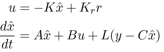
If all states are not measurable, it seems reasonable to try the feedback (5.29)where xˆ is the output of an observer of the state (5.26), i.e.
 (5.30)Since the system (5.28) and the observer (5.30) both are of order n, the closed loop system is thus of order 2n. The states of the system are x and xˆ. The evolution of the states is described by equations (5.28), (5.29)(5.30). To analyze the closed loop system, the state variable xˆ is replace by
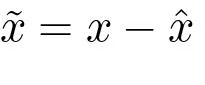 (5.31)
Subtraction of (5.28) from (5.28) gives Introducing u from (5.29) into this equation and using (5.31) to eliminate xˆ gives
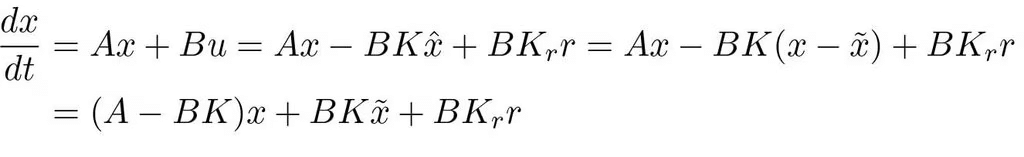
The closed loop system is thus governed by
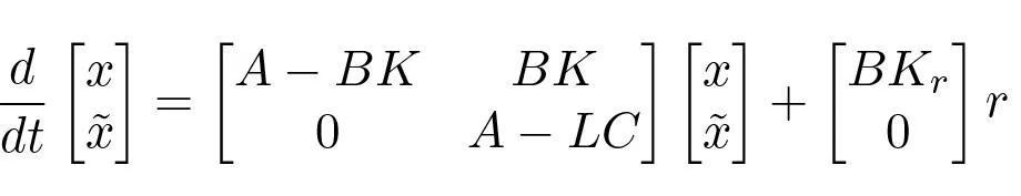 (5.32)
Since the matrix on the right-hand side is block diagonal, we find that the characteristic polynomial of the closed loop system is
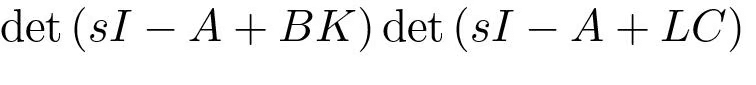
This polynomial combines two parts: one from the closed-loop system with state feedback, and one from the observer error. The feedback in (5.29), based on a simple hunch, nicely solves the eigenvalue placement problem, as summarized below.
Theorem 5.3 (Pole placement by output feedback).
Consider the system:

The controller described by
gives a closed loop system with the characteristic polynomial
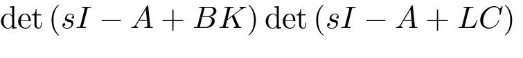 This polynomial can be assigned arbitrary roots if the system is observable and reachable.
Remark 5.5:
It's a 2n-order polynomial, splitting into two parts-one tied to state feedback (det(sI - A + BK)) and one to the observer (det(sI - A + LC)).
Remark 5.6:
The controller feels intuitive, blending state feedback and an observer, with the feedback gain K calculated as if all states are measurable.
The Internal Model Principle
A block diagram of the controller is shown in Figure 5.4. Notice that the controller contains a dynamical model of the plant. This is called the internal model principle. Notice that the dynamics of the controller is due to the observer. The controller can be viewed as a dynamical system with input y and output u.
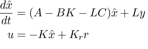 (5.33)
The controller has the transfer function
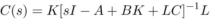 (5.34)
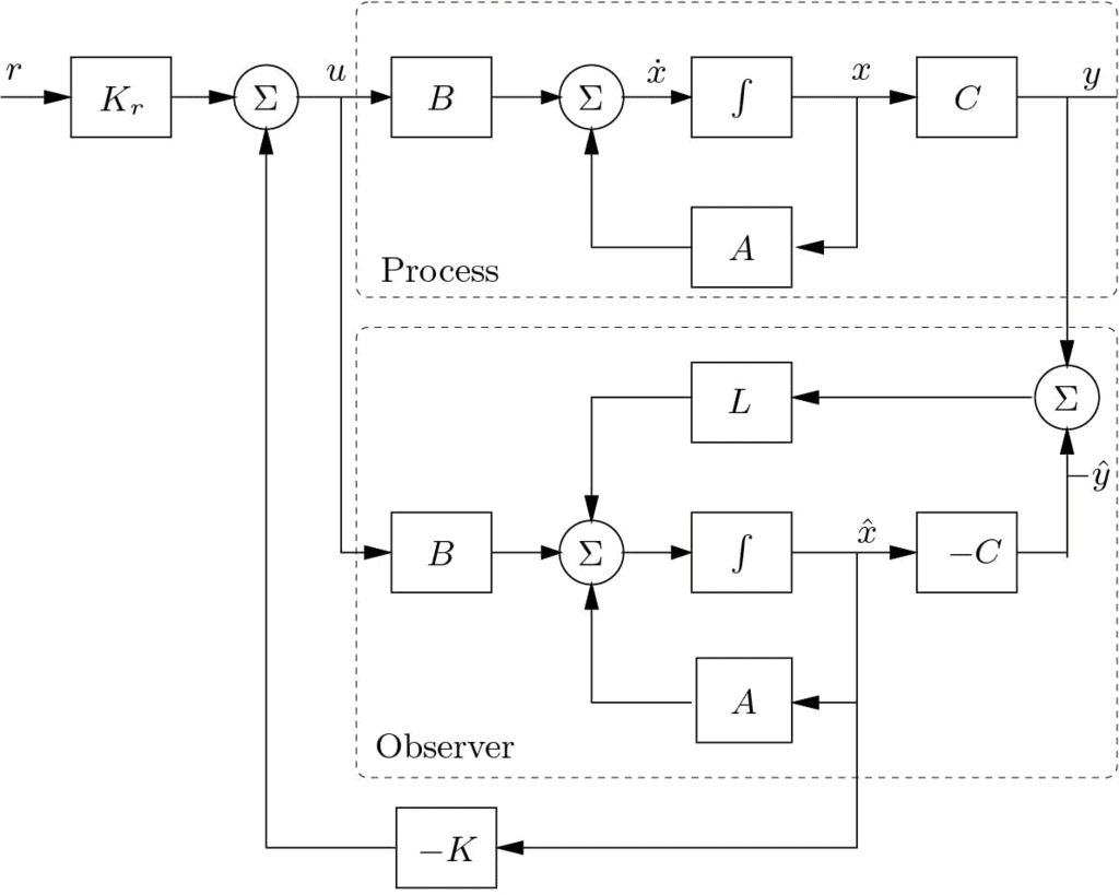 Figure 5.4: Block diagram of a controller which combines state feedback with an observer.
Conclusion
State and output feedback provide a powerful framework for controlling linear systems by shaping their dynamics through eigenvalue placement. State feedback directly uses the system's state to achieve desired behavior when all variables are measurable, while output feedback, paired with an observer, extends this capability to systems where only outputs are available, ensuring effective control by estimating the state and embedding a model of the system within the controller.
FAQs on State and Output Feedback
| 1. What does it mean for a system to be not reachable in control theory? |  |
| 2. How do coordinate changes affect the reachability of a system? | |
| 3. What is the significance of computing the feedback gain in control systems? | |
| 4. Can you explain observability and its relation to control systems? | |
| 5. What does it mean for a system to be non-observable, and how does this impact control design? | |


 | Explore Courses for Electrical Engineering (EE) exam |
 | Get EduRev Notes directly in your Google search |