Describing the Distribution of a Quantitative Variable Chapter Notes | AP Statistics - Grade 9 PDF Download

Once you've organized your data into a visual representation like a histogram, dotplot, or stemplot, the next step is to describe what the data reveals. To effectively analyze a quantitative variable's distribution, focus on three key aspects: shape, center, and spread. Below, we explore these elements in detail to help you uncover patterns and trends in your data.
Shape
The shape of a distribution provides insights into the data's structure. Here are the key features to examine:
Symmetry
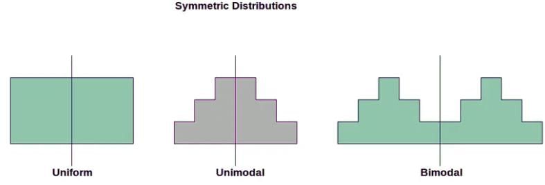
A distribution is symmetric if, when folded along its central value, both sides mirror each other, much like a butterfly's wings. For example, a bell-shaped curve is symmetric because the data on either side of the central point (mean or median) are roughly equivalent. To assess symmetry:
- Visually inspect the histogram to see if the left and right halves are similar.
- Compare statistical measures like the mean and median; in symmetric distributions, they are often close or equal.
Skewness
Skewness describes the asymmetry of a distribution, where one tail is longer than the other:
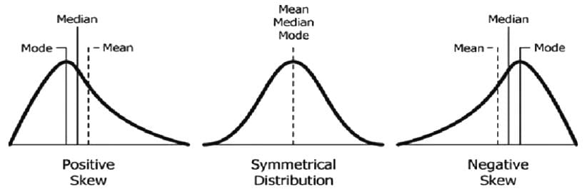
- Right-skewed (Positive Skewness): The tail extends further on the right, with most values clustered on the left and a few larger values stretching to the right. The mean is typically greater than the median.
- Left-skewed (Negative Skewness): The tail is longer on the left, with most values clustered on the right and a few smaller values extending to the left. The mean is typically less than the median.
Peaks (Modes)
A mode is the most frequent value(s) in a dataset, visible as peaks in histograms, stemplots, or dotplots (but not boxplots). Distributions can be:
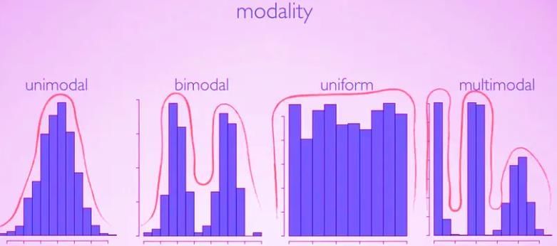
- Unimodal: One peak, indicating a single dominant value.
- Multimodal: Two or more peaks, suggesting multiple subgroups within the data (e.g., a bimodal distribution has two modes).
- Uniform: No distinct peaks, as all values occur with similar frequency.
 Outliers
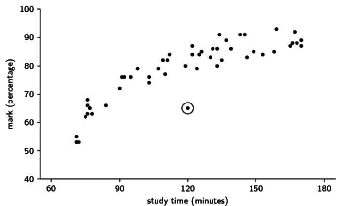
Outliers are data points that significantly deviate from the majority, either being unusually high or low. They can affect measures like the mean, median, and range, so it’s crucial to:
- Use graphical tools like boxplots to spot outliers visually.
- Calculate statistical measures (e.g., mean and standard deviation) to identify extreme values.
- Analyze data with and without outliers to understand their impact.
Gaps
Gaps are intervals in the data with no observations, indicating breaks in the distribution. They can signal multiple modes or distinct data groups, helping you understand variability and potential subpopulations.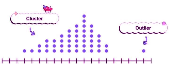
Center
The center of a distribution indicates its typical value. Three common measures are:
- Mean: The average, calculated by summing all values and dividing by the count. Best for symmetric distributions, as it reflects all data points.
- Median: The middle value when data is ordered. Ideal for skewed distributions, as it’s less affected by outliers.
- Mode: The most frequent value, useful when a few values dominate.
In symmetric distributions, the mean, median, and mode are often similar. In skewed distributions or those with outliers, they may differ significantly. Choose the measure that best suits the data’s characteristics.
Spread
Spread describes how much the data varies. Key measures include:
- Range: The difference between the maximum and minimum values. Simple but limited, as it only considers extremes.
- Standard Deviation: Measures dispersion around the mean, calculated as the square root of the variance (average of squared differences from the mean). Ideal for symmetric distributions.
- Interquartile Range (IQR): The range of the middle 50% of data (Q3 - Q1). Robust for skewed distributions or those with outliers.
For symmetric distributions, report the mean and standard deviation. For skewed distributions, use the median and IQR to provide a fuller picture of variability.
Key Vocabulary
Understanding these terms is essential for describing distributions:
- Gaps: Intervals with no data, highlighting variability or distinct groups.
- Histogram: A bar-based graph showing data frequency in intervals, revealing shape, center, and spread.
- Interquartile Range (IQR): The range of the middle 50% of data, resistant to outliers.
- Mean: The average, reflecting the overall trend in symmetric data.
- Median: The middle value, robust for skewed data.
- Mode: The most frequent value, indicating common observations.
- Modes: Multiple frequent values, revealing data clusters.
- Multimodal Distribution: A distribution with multiple peaks, indicating subgroups.
- Outlier: A significantly different data point, affecting statistical measures.
- Range: The difference between maximum and minimum values, showing variability.
- Right-Skew: A distribution with a longer right tail, where the mean exceeds the median.
- Skewness: The degree of asymmetry in a distribution, positive or negative.
- Standard Deviation: A measure of dispersion around the mean.
- Spread: The extent of data variability.
- Symmetry: A balanced distribution where both sides mirror each other.
- Uniform Distribution: A distribution where all values are equally likely, with no distinct modes.
|
12 videos|106 docs|12 tests
|
FAQs on Describing the Distribution of a Quantitative Variable Chapter Notes - AP Statistics - Grade 9
| 1. What is meant by the 'shape' of a distribution in statistics? |  |
| 2. How do we determine the 'center' of a quantitative variable's distribution? | |
| 3. What are some common measures of 'spread' in a distribution? | |
| 4. Why is it important to analyze the distribution of a quantitative variable? | |
| 5. How can skewness affect the interpretation of data in a distribution? | |


practice quizzes
,Describing the Distribution of a Quantitative Variable Chapter Notes | AP Statistics - Grade 9
,past year papers
,Free
,Objective type Questions
,Semester Notes
,mock tests for examination
,shortcuts and tricks
,Describing the Distribution of a Quantitative Variable Chapter Notes | AP Statistics - Grade 9
,Sample Paper
,Describing the Distribution of a Quantitative Variable Chapter Notes | AP Statistics - Grade 9
,Extra Questions
,ppt
,study material
,video lectures
,MCQs
,Previous Year Questions with Solutions
,Summary
,Viva Questions
,Important questions
,Exam
;


Chapter Notes: Describing the Distribution of a Quantitative Variable Free PDF Download
Importance of Chapter Notes: Describing the Distribution of a Quantitative Variable
Chapter Notes: Describing the Distribution of a Quantitative Variable
Chapter Notes: Describing the Distribution of a Quantitative Variable Grade 9 Questions
Study Chapter Notes: Describing the Distribution of a Quantitative Variable on the App
|
© EduRev
|
Education Revolution
|


|


