The Normal Distribution Chapter Notes | AP Statistics - Grade 9 PDF Download

Intro to Z-Scores
This section introduces z-scores. When I think of statistics, standard deviation and z-scores come to mind. So, what exactly are z-scores? A z-score, also known as a standard score, measures how many standard deviations a data point is from the mean (not median) of a data set. It is calculated using the formula:
FORMULA: z = (x - x̄) / s
- z = z-score
- x = a data point
- x̄ = mean value
- s = standard deviation
For example, consider a data set with a mean of 50 and a standard deviation of 10. If a data point has a value of 70, the z-score would be:
z-score = (70 - 50) / 10 = 2
This z-score of 2 means that the data point is 2 standard deviations above the mean of the data set.
Z-scores are useful for:
- Comparing values within a data set
- Determining if a value is unusual or extreme
- Standardizing data for comparison between different data sets
For this reason, z-scores are also called standardized values. In sports, judges often calculate final scores using z-scores.
Negative z-scores indicate that the data value is below the mean, while positive z-scores indicate it is above the mean. The further the value is from the mean, the more unusual it is.
Effect of Standardization on Distribution
When we standardize data into z-scores:
- We shift the data by the mean
- We rescale by the standard deviation
Shifting data changes the distribution's center but keeps its shape and spread unchanged. The center shifts along with other measures like percentiles, minimum, and maximum. Rescaling stretches or squeezes the distribution but alters the mean, minimum, maximum, range, IQR, and standard deviation.
AP Statistics MCQs often ask about how shifting and rescaling affect shape, center, and spread, so be prepared for these questions!
Normal Model: More than Just a Hump
You may have learned about normal models or bell-shaped curves in your Algebra class and through calculus. Some sets of data may be described as approximately normally distributed. A normal curve is mound-shaped and symmetric.
Characteristics of Normal Models
Normal models are suitable for symmetric and unimodal distributions. The normal model has two parameters:
- Population mean (µ)
- Population standard deviation (σ)
It is often written as N(mean, sd). These parameters are part of the model and do not come from the data.
Examples of Normal Distribution in Daily Life
You might be curious about what variables in daily life can be modeled by a normal distribution. Here are some examples:
- Height
- IQ scores
- Blood pressure
- Birth weight
- Body temperature
- Life expectancy
- Income
Standard Normal Model
The standard normal model is represented by a symmetrical, bell-shaped curve, with a mean of 0 and a standard deviation of 1. It is denoted as N(0,1). Z-scores, which are key to understanding this model, help standardize data, making it easier to compare and analyze.
Standardization Process
- To standardize a value, use the formula: z = (x - x̄) / s, where x is the value, x̄ is the mean, and s is the standard deviation.
Conditions for Normality
For data to fit the standard normal model well, it should be:
- Approximately symmetric
- Unimodal (having one peak)
Checking Normality
To assess if the data meets these conditions, it's common to:
- Examine a histogram for symmetry and a single peak.
- Create a normal probability plot.
Always ensure to check the "Nearly Normal" condition before applying the normal model to your data.
The Empirical (68-95-99.7) Rule
Many wonder if their behaviors are typical. The Empirical Rule helps answer this by stating that in a normal distribution:
- About 68% of values fall within 1 standard deviation of the mean.
- About 95% of values fall within 2 standard deviations of the mean.
- About 99.7% of values fall within 3 standard deviations of the mean.
This rule is useful for understanding how data is spread around an average. However, it only applies to normal distributions. For data that is skewed, a different approach, known as Chebyshev’s rule, is needed.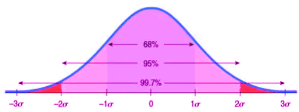
Key Points about the Empirical Rule:
- It describes the spread of values in a bell-shaped curve.
- The inflection point (where the curve changes direction) is found at 1 standard deviation from the mean.
- Do not extend the distribution beyond 3 standard deviations as very few values exist there.
For visualization, when sketching a normal distribution, start with the center and draw the tails outward, ensuring the curve resembles a bell shape.
Key Vocabulary
- Density Curve
- Normal Distribution
- Normal Curve
- The Empirical Rule
- Standard Normal Distribution
- Z-Score
- Normal Probability Plot
Practice Problems
(1) A sample of 50 students at a school took a math test, and the mean score was 75 out of 100. The standard deviation of the scores was 10.
Problem A
- Calculate the z-score for a student who scored a 90 on the test.
Problem B
- Interpret the z-score. What does this mean in the context of statistics and test scores?
(2) A baseball player has a batting average of 0.300, which is the mean number of hits per at-bat over the course of a season. The standard deviation of the player's batting average is 0.050. In a recent game, the player had 4 at-bats and scored 3 hits.
Problem
- Calculate the z-score for the player's performance in this game.
(3) Another big idea within Unit 1 of the AP Stats course is the idea that percentiles and z-scores may be used to compare relative positions of points within a data set or between data sets.
Study Example
A study was conducted to determine the average number of hours per week that college students spend studying. The study found that:
- The average number of hours per week spent studying is 15 hours.
- The standard deviation is 4 hours.
A random sample of 25 college students was selected, and the sample mean was found to be 13 hours per week, with a z-score of -1.5.
Ans:
(1) Calculating the Z-Score for a Student's Test Score
- First, find the difference between the student's score and the mean score: 90 - 75 = 15
- Next, divide this difference by the standard deviation: 15 / 10 = 1.5
- The z-score is 1.5, indicating the student scored 1.5 standard deviations above the mean.
- Note: Ensure all values (mean, standard deviation, and score) are in the same units (e.g., points).
(2) Calculating the Z-Score for a Player's Batting Average
- Calculate the batting average: 3 hits / 4 at-bats = 0.750
- Find the difference from the mean batting average: 0.750 - 0.300 = 0.450
- Divide by the standard deviation: 0.450 / 0.050 = 9
- The z-score is 9, indicating an exceptional performance.
(3) Finding the Average Study Hours of College Students
- Use the z-score formula: z = (x - x̄) / standard deviation
- Given mean = 15 hours, standard deviation = 4 hours, and z-score = -1.5.
- Substituting values into the formula gives: -1.5 = (x - 15) / 4
- Multiply both sides by 4: -6 = x - 15
- Adding 15 results in: x = 9
- The average study hours per week for college students is 9 hours.
Key Terms to Review (8)
Density Curve
- A density curve visually represents the distribution of a continuous random variable.
- It must always lie on or above the horizontal axis, with the total area equaling one, representing total probability.
- Helps in understanding the likelihood of different outcomes, especially in contexts like random variables and distributions like the normal distribution.
Empirical Rule
- The Empirical Rule (68-95-99.7 rule) states that in a normal distribution:
- Approximately 68% of data falls within one standard deviation from the mean.
- About 95% falls within two standard deviations.
- Around 99.7% falls within three standard deviations.
- Crucial for understanding data spread in statistical analyses.
Normal Probability Plot
- A Normal Probability Plot checks if a data set follows a normal distribution.
- Data points plotted against expected values can show deviations from normality.
- A straight line indicates a normal distribution; points close to it suggest normality.
Normal Distribution
- Normal distribution is a continuous probability distribution with a symmetric, bell-shaped curve.
- Most observations cluster around the central peak, with probabilities tapering off equally on both sides.
- This concept is foundational in statistics, influencing many statistical tests and methods.
Standardize
- To standardize means converting a data point into a standardized score (z-score).
- This allows comparison across datasets by indicating how many standard deviations a value is from the mean.
Standard Normal Model
- The Standard Normal Model is a normal distribution with a mean of 0 and a standard deviation of 1.
- It simplifies calculations and comparisons across different normal distributions.
Symmetrical Bell-Shaped Curve
- The symmetrical bell-shaped curve represents data evenly distributed around a central mean.
- Its symmetric shape shows that most data points cluster around the mean.
- Understanding this curve is essential for probability calculations and inferential statistics.
Z-Score
- A Z-score indicates how many standard deviations a data point is from the mean.
- It helps in comparing data points from different distributions.
|
12 videos|106 docs|12 tests
|
FAQs on The Normal Distribution Chapter Notes - AP Statistics - Grade 9
| 1. What is the empirical rule in the context of the normal distribution? |  |
| 2. How can the empirical rule be used in real-life scenarios? | |
| 3. What does it mean if data does not follow a normal distribution? | |
| 4. Can the empirical rule be applied to non-normal distributions? | |
| 5. What are some common misconceptions about the normal distribution? | |


Viva Questions
,mock tests for examination
,video lectures
,Sample Paper
,The Normal Distribution Chapter Notes | AP Statistics - Grade 9
,Extra Questions
,Summary
,MCQs
,Important questions
,The Normal Distribution Chapter Notes | AP Statistics - Grade 9
,The Normal Distribution Chapter Notes | AP Statistics - Grade 9
,Semester Notes
,Objective type Questions
,Free
,past year papers
,study material
,Previous Year Questions with Solutions
,practice quizzes
,Exam
,ppt
,shortcuts and tricks
;


Chapter Notes: The Normal Distribution Free PDF Download
Importance of Chapter Notes: The Normal Distribution
Chapter Notes: The Normal Distribution
Chapter Notes: The Normal Distribution Grade 9 Questions
Study Chapter Notes: The Normal Distribution on the App
|
© EduRev
|
Education Revolution
|


|


