Residuals Chapter Notes | AP Statistics - Grade 9 PDF Download

When evaluating the effectiveness of a linear regression model, we use residuals to assess its accuracy.
What is a Residual?
Residuals measure how well a linear regression model fits the data. They are calculated as the difference between the observed values of the response variable (y) and the predicted values from the model (ŷ), expressed as:
- Residual: y - ŷ
Understanding Residuals
The goal of a linear regression model is to find the line of best fit that minimizes the sum of the squared residuals. This approach is known as the least squares criterion. Each residual represents the vertical distance between a data point and the line of best fit:
- If a point has a small residual, the model predicts the response variable well.
- If a point has a large residual, the model does not predict the response variable well.
Positive and Negative Residuals
Residuals can be categorized as positive or negative:
- A positive residual indicates that the actual value is greater than the predicted value, meaning the model underestimates the true value.
- A negative residual indicates that the actual value is less than the predicted value, meaning the model overestimates the true value.
Residual Plots
A residual plot is a type of graph that displays the residuals— the differences between observed values and predicted values. In these plots:
- The vertical axis shows the residuals.
- The horizontal axis represents the predictor or explanatory variable.
Understanding Residual Plots
If the residual plot for a linear regression model shows apparent randomness, it suggests that the relationship between the predictor and response variables is likely linear. This means:
- The model is effectively capturing the underlying relationship in the data.
- Residuals are randomly scattered around the horizontal axis.
- There is no systematic relationship between the residuals and the predictor variable.
Below are examples of scatterplots with linear regression models and their respective residual plots.
Examples of Linear Regression and Residuals
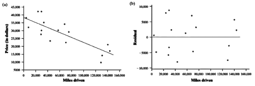
Example 1
In this example, our linear regression model fits the data well, as shown in the scatterplot on the left. The corresponding residual plot on the right reveals no clear pattern, indicating that the model is appropriate. The red points are evenly distributed around the red line at zero.
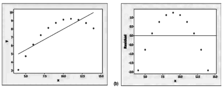
 Example 2
Here, the data exhibits a curved pattern rather than a linear one, as seen in the left scatterplot. Consequently, the residual plot on the right displays an evident curve, suggesting the need for a different model. We will explore how to adapt these models in Unit 2.9.
Good or Bad?
To determine if a model is good, examine the residual plot. For a good model, the residuals should be randomly scattered, showing no clear pattern. In contrast, if the plot shows a distinct curve, as seen in the second set, a linear regression model is not suitable; instead, a nonlinear model would be more appropriate.
Calculating Residuals
To calculate a residual for a specific data point, follow these steps:
Steps to Calculate Residuals
- Obtain the Least Squares Regression Line (LSRL) for the dataset.
- Calculate the predicted value using the LSRL.
- Use the formula: Residual = (Actual) - (Predicted).
This formatted HTML organizes the content clearly and highlights the key points while maintaining readability.
Example 1
A LSRL model for the predicted amount of Lucky Charms eaten based on age is given by the equation:
= 150.5x - 2.34
A 50-year-old from our data set is reported to have eaten 7,500 Lucky Charms in his life. Wow! I hope he found the gold at the end of the rainbow!
Calculate the Residual
Using the equation:
- = 150.5(50) - 2.34
- = 7522.66
To find the residual:
- Residual = Actual value - Predicted value
- Residual = 7500 - 7522.66 = -22.66
Keep in mind that you may sometimes need to calculate the actual data point (or predicted data point) when given the residual. This will involve using the same formula but working backwards.
Example 2
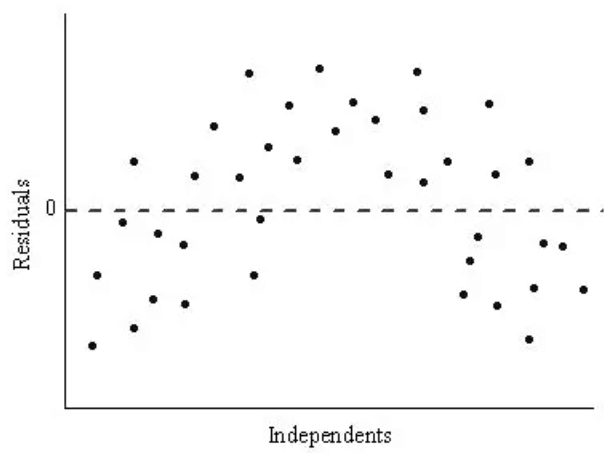
A researcher is studying how the number of hours students spend studying affects their exam scores. She collects data from 50 students and creates a linear regression model. The residual plot for this model shows the difference between the actual scores and the predicted scores.
Questions
a) Describe the pattern, if any, in the residual plot.
b) Explain what the pattern in the residual plot suggests about the fit of the model.
c) If the model is not fitting the data well, suggest one potential reason why this may be the case.
d) Assuming that the model is not fitting the data well, propose one potential solution to improve the fit of the model.
e) Explain how the solution you proposed in part (d) would address the issue with the model.
Answers
a) The residual plot shows a curved pattern.
b) This curved pattern indicates that the model's fit is poor, as the residuals are not randomly scattered. There is likely a systematic relationship between the variables that the model isn't capturing.
c) One potential reason for the poor fit is that the relationship between study hours and exam scores may not be linear; other factors might be influencing the results.
d) A potential solution to improve the model's fit could be to transform the data, such as by taking the logarithm of the study hours or exam scores.
e) This transformation could help reveal a more accurate relationship between the variables, potentially leading to a better model fit by aligning the data with a more suitable functional form.
Key Terms to Review
- Least Squares Criterion: The least squares criterion is a statistical method used to find the best-fitting line through a set of data points. It minimizes the sum of the squares of the differences (residuals) between observed values and predicted values, ensuring the line is positioned to reduce overall discrepancies.
- Linear Regression Model: A linear regression model describes the relationship between a dependent variable and one or more independent variables by fitting a linear equation to observed data. This model is crucial for predicting outcomes and understanding trends.
- LSRL (Least Squares Regression Line): The Least Squares Regression Line (LSRL) finds the line that minimizes the sum of the squares of the vertical distances (residuals) from observed data points to the line, allowing for predictions based on the relationship between two variables.
- Nonlinear Model: A nonlinear model represents relationships that cannot be expressed as a straight line, often resulting in curves or complex patterns. Understanding these models is essential for interpreting data that defies linear assumptions.
- Predicted Values: Predicted values are outcomes generated by a statistical model for given inputs. They estimate responses based on identified relationships in the data, crucial for evaluating model accuracy through residuals.
- Predictor Variable: A predictor variable (or independent variable) is used in analysis to predict the value of another variable (dependent variable). It serves as an input that influences the output, helping researchers assess relationships.
- Randomness: Randomness indicates a lack of predictability in events. It is vital in statistics for understanding variability and drawing conclusions from data, essential for accurate modeling and predictions.
- Residual Plot: A residual plot shows residuals on the vertical axis and the independent variable on the horizontal axis. It helps assess how well a regression model fits data by revealing patterns in residuals.
- Residuals: Residuals are the differences between observed and predicted values in a regression model. They are crucial for assessing model fit and understanding prediction errors.
- Response Variable: A response variable is the main variable being studied to determine its relationship with others. It reflects outcomes influenced by independent variables, providing insights for predictions.
- Scatterplot: A scatterplot visualizes values for two quantitative variables using dots for individual data points, helping identify patterns, trends, and correlations between variables.
|
12 videos|106 docs|12 tests
|
FAQs on Residuals Chapter Notes - AP Statistics - Grade 9
| 1. What are residuals in regression analysis? |  |
| 2. How can residual plots help in assessing the goodness of fit? | |
| 3. What are the common patterns to look for in a residual plot? | |
| 4. How do you interpret a residual plot that shows a random pattern? | |
| 5. What should you do if you notice a pattern in the residual plot? | |


past year papers
,shortcuts and tricks
,Residuals Chapter Notes | AP Statistics - Grade 9
,Residuals Chapter Notes | AP Statistics - Grade 9
,Objective type Questions
,mock tests for examination
,ppt
,Previous Year Questions with Solutions
,Sample Paper
,Summary
,Residuals Chapter Notes | AP Statistics - Grade 9
,Viva Questions
,MCQs
,practice quizzes
,video lectures
,Free
,Exam
,Extra Questions
,Semester Notes
,study material
,Important questions
;


Chapter Notes: Residuals Free PDF Download
Importance of Chapter Notes: Residuals
Chapter Notes: Residuals
Chapter Notes: Residuals Grade 9 Questions
Study Chapter Notes: Residuals on the App
|
© EduRev
|
Education Revolution
|


|


