The Geometric Distribution Chapter Notes | AP Statistics - Grade 9 PDF Download

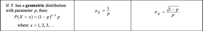
A geometric random variable is a type of discrete random variable that models the number of trials needed to achieve the first success in a sequence of independent trials. Each trial has two possible outcomes: success or failure, with probability p and 1 - p, respectively. The probability distribution of Y is a geometric distribution with probability p of success on any trial, where the possible values of Y are 1, 2, 3, …, n.
For example, suppose you are trying to find the number of coin flips needed to get the first heads. In this case, X is a geometric random variable that represents the number of flips needed to get the first heads. The probability of success (getting a heads) is p = 0.5, and the probability of failure (getting a tails) is 1 - p = 0.5.
Binomial vs. Geometric: Spot the Difference!
Wait, but doesn't the description above look exactly like the set-up for binomial distributions?
Well, the main difference between binomial and geometric random variables is the type of outcome they are used to model:
- A binomial random variable is used to model the number of successes in a fixed number of trials.
- A geometric random variable is used to model the number of trials needed to achieve the first success.
Examples:
Situation 1: Flipping a coin 10 times and counting the number of heads.
In this example, you are performing a fixed number of trials (10 flips) and counting the number of successes (heads). The random variable X would be a binomial random variable with parameters n = 10 and p = 0.5 (assuming the coin is fair).
Situation 2: Flipping a coin until you get the first heads.
In this situation, you are performing a sequence of trials (coin flips) until you achieve the first success (heads). The random variable X would be a geometric random variable with probability p = 0.5 (assuming the coin is fair).
Calculating Probabilities
If a random variable Y follows a geometric distribution with probability p of success on each trial, then the possible values of Y are 1, 2, 3, ..., representing the number of trials needed to achieve the first success. To calculate the probability of a specific value k, you can use the probability function of the geometric distribution:
P(Y=k) = (1-p)^(k-1) * p
For example, if Y is a geometric random variable with probability p = 0.5 of success on each trial, then the probability of Y being equal to 3 (that is, the probability of needing 3 trials to achieve the first success) is:
P(Y=3) = (1-p)^(3-1) * p = (1-0.5)^(3-1) * 0.5 = 0.25 * 0.5 = 0.125
You can also use the cumulative distribution function (CDF) or the probability density function (PDF) of the geometric distribution to calculate probabilities. When using technology, the CDF of the geometric distribution (geometric CDF) gives the probability of Y being less than or equal to a specific value k, while the PDF (geometric PDF) gives the probability of Y being equal to a specific value k.
Shape, Center, and Variability
The mean and standard deviation of a geometric random variable Y can be calculated using the following formulas:
- Mean -- The mean (expected value) of a geometric random variable Y, which represents the number of trials needed to achieve the first success with probability p of success on each trial, is given by: mean = E(Y) = 1/p
- Standard deviation -- The standard deviation of a geometric random variable Y, which represents the number of trials needed to achieve the first success with probability p of success on each trial, is given by: standard deviation = σY = sqrt((1-p)/p)
Every geometric distribution has a skewed right graph, meaning that the graph of the distribution is skewed towards the right side of the mean. This is due to the fact that the geometric random variable can take on only positive integer values, and the probability of success decreases as the number of trials increases. ➡️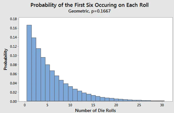
Practice Problem
A manufacturing company produces a product that has a 5% defect rate. This means that the probability of a product being defective is p = 0.05. The company wants to know the probability of the first defective product being produced on the 20th unit. What is the probability of the first defective product being produced on the 20th unit?
Answer: To solve this problem, we can use the probability function of a geometric random variable. The probability function gives the probability of the first success occurring on the nth trial, where the probability of success is p.
In this case, Y is a geometric random variable that represents the number of units needed to produce the first defective product. The probability of success (producing a defective product) is p = 0.05, and the probability of failure (producing a non-defective product) is 1 - p = 0.95.
To find the probability of the first defective product being produced on the 20th unit, we use the probability mass function:
P(Y=20) = (1-p)^(20-1) * p
= (1-0.05)^(20-1) * 0.05
= (0.95^19) * 0.05
= 0.0189
Interpretation in Context: This means that the probability of the first defective product being produced on the 20th unit is about 0.0189, or 1.89%.
Key Terms to Review
- Binomial Random Variable: A type of discrete random variable that counts the number of successes in a fixed number of independent Bernoulli trials, each with the same probability of success.
- Cumulative Distribution Function (CDF): Describes the probability that a random variable takes on a value less than or equal to a specific value.
- Geometric Distribution: Models the number of trials required for the first success in a series of independent Bernoulli trials.
- Geometric Random Variable: Counts the number of trials until the first success occurs in a series of independent Bernoulli trials.
- Probability Mass Function (PMF): Provides the probabilities of discrete random variables, assigning a probability to each possible value.
- Skewed Right Graph: Indicates that most data points are concentrated on the left side, with a tail extending towards the right.
- Standard Deviation: A measure of the amount of variation or dispersion in a set of values.
|
12 videos|106 docs|12 tests
|
FAQs on The Geometric Distribution Chapter Notes - AP Statistics - Grade 9
| 1. What is the main difference between a binomial random variable and a geometric random variable? |  |
| 2. How do you calculate the probability of a specific value k in a geometric distribution? | |
| 3. What is the expected value (mean) of a geometric random variable, and how is it calculated? | |
| 4. What does it mean if a geometric distribution has a skewed right graph? | |
| 5. How do you interpret the probability of the first defective product being produced on the 20th unit? | |


Sample Paper
,Summary
,Important questions
,Viva Questions
,shortcuts and tricks
,ppt
,Exam
,MCQs
,Extra Questions
,practice quizzes
,The Geometric Distribution Chapter Notes | AP Statistics - Grade 9
,Semester Notes
,mock tests for examination
,past year papers
,video lectures
,Previous Year Questions with Solutions
,The Geometric Distribution Chapter Notes | AP Statistics - Grade 9
,The Geometric Distribution Chapter Notes | AP Statistics - Grade 9
,Objective type Questions
,Free
,study material
;


Chapter Notes: The Geometric Distribution Free PDF Download
Importance of Chapter Notes: The Geometric Distribution
Chapter Notes: The Geometric Distribution
Chapter Notes: The Geometric Distribution Grade 9 Questions
Study Chapter Notes: The Geometric Distribution on the App
|
© EduRev
|
Education Revolution
|


|


