Measures of Central Tendency Chapter Notes | Mathematics Class 10 ICSE PDF Download

Introduction
Imagine you're trying to summarize a big pile of data, like the heights of all students in your school or the scores in a class test. Measures of central tendency are like the "middle ground" that help us describe the typical or central value in such data sets. These measures give us a single number that represents the whole group, making it easier to understand and compare data. They are designed to capture the essence of the data by focusing on a value that's neither too high nor too low but somewhere in the middle where most data points tend to cluster. This chapter dives into four key measures: mean, median, quartiles, and mode, each offering a unique way to summarize data!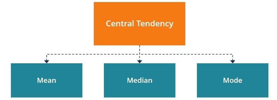
- Measures of central tendency are numerical values that represent the characteristics of a large data set.
- They provide a central value that lies between the highest and lowest values, often where most data points are concentrated.
- The chapter covers:
- Arithmetic Mean
- Median
- Mode
- Quartiles
Arithmetic Mean
- The arithmetic mean, or simply mean, is the sum of all numbers in a set divided by the count of numbers.
- It represents the average value of the data set.
- Formula: Mean = (x1 + x2 + x3 + ... + xn) / n = Σx / n,
- where Σ (sigma) denotes the sum of numbers, and n is the number of terms.
- Steps to calculate:
- Add all the numbers in the data set (Σx).
- Count the total number of values (n).
- Divide the sum by the number of values to get the mean.
- Sum of weights = 67 + 65 + 71 + 57 + 45 = 305 kg
- Number of persons (n) = 5
- Mean = Σx / n = 305 / 5 = 61 kg
- Answer: The arithmetic mean is 61 kg.
Arithmetic Mean of Tabulated Data
For data presented in a frequency distribution table, the mean can be calculated using three methods:
- Direct Method
- Short-cut Method
- Step-deviation Method
1. Direct Method
- Uses the frequency of each value to calculate the mean.
- Formula: Mean = Σ(fx) / Σf, where f is the frequency, x is the variate, and Σf is the total frequency.
- Steps:
- Create a table with columns for variate (x), frequency (f), and product (fx).
- Multiply each variate by its frequency to get fx.
- Sum the frequencies (Σf) and the products (Σfx).
- Calculate mean by dividing Σfx by Σf.
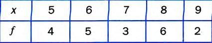 Solution:
Create a table:
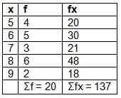
Mean = Σfx / Σf = 137 / 20 = 6.85
Answer: The mean is 6.85.2. Short-cut Method
- Simplifies calculations by using an assumed mean (A).
- Formula: Mean = A + (Σfd / Σf), where d = x - A (deviation from assumed mean).
- Steps:
- Create a table with columns for x, f, d = x - A, and fd.
- Choose an assumed mean (A), preferably a central value of x.
- Calculate deviations (d) by subtracting A from each x.
- Multiply each d by its frequency to get fd.
- Sum the frequencies (Σf) and the products (Σfd).
- Apply the formula to find the mean.
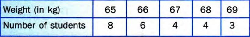 Find the mean using the short-cut method.
Solution:
Let assumed mean A = 67.
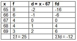
Mean = A + (Σfd / Σf) = 67 + (-12 / 25) = 67 - 0.48 = 66.52 kg
Answer: The mean weight is 66.52 kg.3. Step-deviation Method
- Further simplifies calculations by scaling deviations.
- Formula: Mean = A + (Σft / Σf) × i, where t = (x - A) / i, and i is the common factor (largest number dividing all deviations).
- Steps:
- Create a table with columns for x, f, d = x - A, t = d / i, and ft.
- Choose an assumed mean (A).
- Calculate deviations (d = x - A).
- Choose i, the largest number dividing all d values.
- Calculate t = d / i for each variate.
- Multiply each t by its frequency to get ft.
- Sum the frequencies (Σf) and the products (Σft).
- Apply the formula to find the mean.
x: 10, 30, 50, 70, 90, 110
frequency: 135, 187, 240, 273, 124, 151
Solution:
Let A = 70, i = 20 (since deviations are divisible by 20).
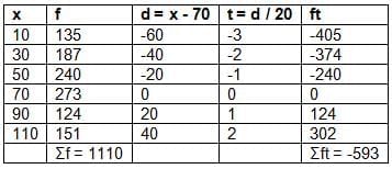
Mean = A + (Σft / Σf) × i = 70 + (-593 / 1110) × 20 = 70 - 10.68 = 59.32
Answer: The mean is 59.32.To Find Mean for Grouped Data (both continuous and discontinuous)
- Grouped data is organized into class intervals, and the mean is calculated using the mid-value of each interval.
- Three methods are used: Direct, Short-cut, and Step-deviation.
1. Direct Method
- Uses mid-values of class intervals as variates.
- Formula: Mean = Σ(fx) / Σf, where x is the mid-value of each class interval.
- Steps:
- Calculate the mid-value (x) of each class interval: x = (lower limit + upper limit) / 2.
- Create a table with columns for class interval, frequency (f), mid-value (x), and fx.
- Multiply each mid-value by its frequency to get fx.
- Sum the frequencies (Σf) and the products (Σfx).
- Calculate mean by dividing Σfx by Σf.
C.I. : 0-10, 10-20, 20-30, 30-40, 40-50
frequency: 10, 6, 8, 12, 5
Solution: C.I and f are given.
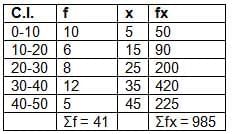
Mean = Σfx / Σf = 985 / 41 ≈ 24.02
Answer: The mean is approximately 24.02.2. Short-cut Method
- Uses an assumed mean to simplify calculations.
- Formula: Mean = A + (Σfd / Σf), where d = x - A, and x is the mid-value.
- Steps:
- Calculate mid-values (x) for each class interval.
- Choose an assumed mean (A), preferably a central mid-value.
- Calculate deviations (d = x - A).
- Multiply each d by its frequency to get fd.
- Sum the frequencies (Σf) and the products (Σfd).
- Apply the formula to find the mean.
C.I.: 35-40, 40-45, 45-50, 50-55, 55-60
frequency: 7, 6, 9, 5, 3
Solution:
Let A = 47.5.
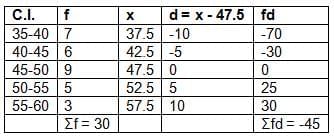
Mean = A + (Σfd / Σf) = 47.5 + (-45 / 30) = 47.5 - 1.5 = 46
Answer: The mean is 46.3. Step-deviation Method
- Uses scaled deviations to simplify calculations.
- Formula: Mean = A + (Σft / Σf) × i, where t = (x - A) / i, and i is the class size.
- Steps:
- Calculate mid-values (x) for each class interval.
- Choose an assumed mean (A).
- Calculate deviations (d = x - A).
- Choose i, the class size (upper limit - lower limit).
- Calculate t = d / i.
- Multiply each t by its frequency to get ft.
- Sum the frequencies (Σf) and the products (Σft).
- Apply the formula to find the mean.
Weight: 80-85, 85-90, 90-95, 95-100, 100-105, 105-110, 110-115
frequency: 5, 8, 10, 12, 8, 4, 3
Solution:
Let A = 97.5, i = 5.

Mean = A + (Σft / Σf) × i = 97.5 + (-16 / 50) × 5 = 97.5 - 1.6 = 95.9 ≈ 96 g
Answer: The mean weight is 96 g (to the nearest gram).Median
- The median is the middle value when data is arranged in ascending or descending order.
- It divides the data into two equal parts.
Median for Raw Data
- For raw data, arrange the values in ascending or descending order and find the middle term.
- Formulas:
- If n is odd: Median = ((n + 1) / 2)th term
- If n is even: Median = [((n / 2)th term + ((n / 2) + 1)th term) / 2]
- Steps:
- Arrange data in ascending or descending order.
- Determine if n is odd or even.
- Apply the appropriate formula to find the median.
Solution:
Arrange in ascending order: 3, 4, 7, 8, 10
n = 5 (odd)
Median = ((5 + 1) / 2)th term = 3rd term = 7
Answer: The median is 7.
Median for Tabulated Data
- For frequency distribution data, use cumulative frequency to find the median.
- Steps:
- Create a cumulative frequency table.
- Find n, the total frequency.
- If n is odd, Median = ((n + 1) / 2)th term.
- Identify the value corresponding to the ((n + 1) / 2)th term using cumulative frequency.
 Find the median weight.
Solution:
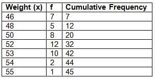
n = 45 (odd)
Median = ((45 + 1) / 2)th term = 23rd termFrom the table, the 21st to 32nd children have weight 52 kg.
Thus, the 23rd term = 52 kg.
Answer: The median weight is 52 kg.
Median for Grouped Data (both continuous and discontinuous)
- For grouped data, the median is estimated using an ogive (cumulative frequency curve).
- Steps:
- Create a cumulative frequency table.
- Plot class intervals on the x-axis and cumulative frequencies on the y-axis.
- Draw a smooth curve (ogive) through the points, starting from the lower limit of the first class to the upper limit of the last class.
- Find n, the total frequency.
- Locate the ((n / 2)th or ((n + 1) / 2)th term on the y-axis, draw a horizontal line to the ogive, then a vertical line to the x-axis to find the median.
C.I. : 0-10, 10-20, 20-30, 30-40, 40-50
frequency: 5, 7, 10, 8, 5
Solution:
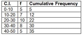
n = 35 (odd)
Median = ((35 + 1) / 2)th term = 18th termPlot points (10, 5), (20, 12), (30, 22), (40, 30), (50, 35) and draw an ogive.
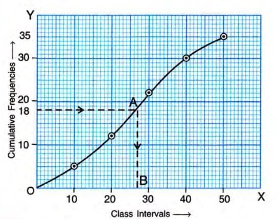 From 18 on the y-axis, draw a horizontal line to the ogive, then a vertical line to the x-axis, which gives approximately 27.
Answer: The median is 27, and the median class is 20-30.
Quartiles
- Quartiles divide a data set into four equal parts when arranged in ascending order.
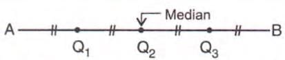
- Lower quartile (Q1): Divides the lower half of the data into two equal parts.
- Middle quartile (Q2): Same as the median.
- Upper quartile (Q3): Divides the upper half of the data into two equal parts.
- Formulas:
- If n is odd: Q1 = ((n + 1) / 4)th term, Q3 = (3(n + 1) / 4)th term
- If n is even: Q1 = (n / 4)th term, Q3 = (3n / 4)th term
- Steps:
- Arrange data in ascending order.
- Determine if n is odd or even.
- Apply the appropriate formula to find Q1 and Q3.
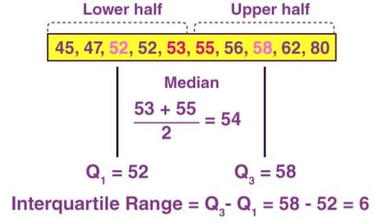
Solution:
Arrange in ascending order: 7, 9, 11, 13, 15, 17, 19
n = 7 (odd)
Q1 = ((7 + 1) / 4)th term = 2nd term = 9
Q3 = (3(7 + 1) / 4)th term = 6th term = 17
Inter-quartile range = Q3 - Q1 = 17 - 9 = 8
Answer: Q1 = 9, Q3 = 17, Inter-quartile range = 8.
Inter-quartile Range
- The inter-quartile range is the difference between the upper and lower quartiles.
- Formula: Inter-quartile range = Q3 - Q1
- It measures the spread of the middle 50% of the data.
Mode
- The mode is the value that occurs most frequently in a data set.
- It represents the point of maximum frequency.
1. Mode for Raw Data
- Identify the value that appears most often in the data set.
- Steps:
- List all values in the data set.
- Count the frequency of each value.
- The value with the highest frequency is the mode.
Solution:
Count frequencies: 4 (3 times), 7 (4 times), 3 (1 time), 2 (1 time), 6 (1 time), 8 (1 time).
The value 7 occurs most frequently.
Answer: The mode is 7.
2. Mode for Tabulated Data
Identify the value with the highest frequency in the frequency distribution table.- Steps:
- Examine the frequency column in the table.
- The value (x) corresponding to the highest frequency is the mode.
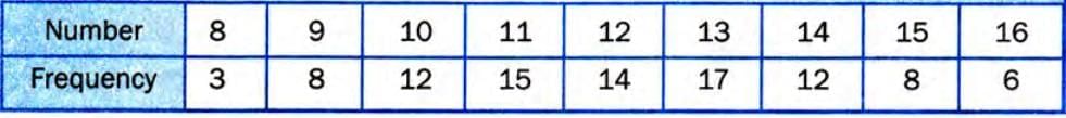 Solution:
The highest frequency is 17, corresponding to the number 13.
Answer: The mode is 13.
3. Mode for Grouped Data
- For grouped data, the mode is estimated using a histogram.
- The modal class is the class interval with the highest frequency.
- Steps:
- Draw a histogram of the frequency distribution.
- Identify the rectangle with the highest height (modal class).
- Draw two diagonal lines from the upper corners of the adjacent rectangles to intersect within the modal class rectangle.
- Draw a perpendicular line from the intersection point to the x-axis.
- The value on the x-axis is the mode.
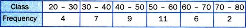 Solution:
The modal class is 50-60 (frequency = 11).
Using a histogram, draw diagonals from the upper corners of the 40-50 and 60-70 rectangles to intersect within the 50-60 rectangle. Drop a perpendicular to the x-axis, which gives approximately 53.
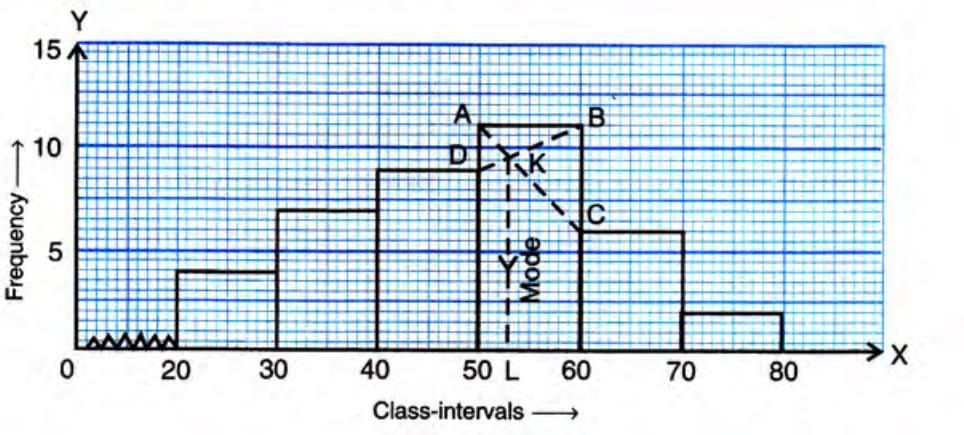 Answer: The mode is 53, and the modal class is 50-60.
|
74 videos|328 docs|30 tests
|
FAQs on Measures of Central Tendency Chapter Notes - Mathematics Class 10 ICSE
| 1. What is the arithmetic mean, and how is it calculated for ungrouped data? |  |
| 2. How do you find the arithmetic mean for grouped data? | |
| 3. What is the median, and how is it determined for raw data? | |
| 4. How can the median be calculated for grouped data? | |
| 5. What are quartiles, and how do you calculate the inter-quartile range? | |


video lectures
,shortcuts and tricks
,past year papers
,Exam
,Extra Questions
,Objective type Questions
,Viva Questions
,ppt
,mock tests for examination
,practice quizzes
,Summary
,Previous Year Questions with Solutions
,Semester Notes
,Measures of Central Tendency Chapter Notes | Mathematics Class 10 ICSE
,Measures of Central Tendency Chapter Notes | Mathematics Class 10 ICSE
,Measures of Central Tendency Chapter Notes | Mathematics Class 10 ICSE
,Sample Paper
,Free
,MCQs
,study material
,Important questions
;


Chapter Notes: Measures of Central Tendency Free PDF Download
Importance of Chapter Notes: Measures of Central Tendency
Chapter Notes: Measures of Central Tendency
Chapter Notes: Measures of Central Tendency Class 10 Questions
Study Chapter Notes: Measures of Central Tendency on the App
|
© EduRev
|
Education Revolution
|


|


