Hashing

Table of Contents
1. Hashing
2. Basic Operations
3. Search Operation
4. Insert Operation
5. Delete Operation
6. Load Factor, Complexity and Rehashing
7. Properties of a Good Hash Function
8. Applications
View more

Hash Table is a data structure which stores data in an associative manner. In a hash table, data are stored in an array, where each data value is placed at an index computed from its key. Access to data becomes very fast if we know the index of the desired data.

Hash tables provide very fast insertion and search operations irrespective of the size of the data, when a suitable hashing method and collision-resolution scheme are used. A hash table uses an array as storage and a hash function to compute the index at which an element should be inserted or searched for.

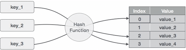
Hashing

Hashing is a technique to convert a (typically large) range of key values into a (smaller) range of array indices. A simple and commonly used hash function for integer keys is the division method, which uses the modulo operator:

index = key % SIZE

Example: consider a hash table of size 20. The following items (in the format (key, value)) are to be stored.

• (1, 20)
• (2, 70)
• (42, 80)
• (4, 25)
• (12, 44)
• (14, 32)
• (17, 11)
• (13, 78)
• (37, 98)

Collision

A collision occurs when two different keys map to the same array index. Collisions are inevitable when the key space is larger than the table size. A collision-resolution strategy is required to handle such cases and still provide efficient operations.

Linear Probing (Open Addressing)

Linear probing is an open addressing collision-resolution method. If the computed index is already occupied, linear probing searches the next cell (index+1), then index+2, and so on, wrapping around the table, until an empty cell is found.

Continuing the previous example, using linear probing to place items results in the following final indices:

Notes about linear probing:

• Linear probing can cause primary clustering: long runs of consecutive occupied slots form and may increase probe lengths.
• Insertion and search probe sequences are identical for a given key, so maintaining deleted slots requires care (see Delete below).

Other Collision-Resolution Methods

• Chaining (Separate Chaining) - each table index stores a pointer to a linked list (or other container) of entries that hash to the same index. Insertions append to the list. This allows the table size to remain fixed while handling arbitrary numbers of keys.
• Quadratic probing - a form of open addressing where the probe sequence is index + c1·i + c2·i² (i = probe number). It reduces primary clustering but may have other trade-offs and requires careful choice of table size.
• Double hashing - uses a second hash function to compute the probe step size; probe sequence becomes index + i·h2(key). Double hashing tends to produce good probe distribution and avoids clustering better than linear probing.

Basic Operations

The primary operations supported by a hash table are:

• Search - find an element given its key.
• Insert - add an element (key, value) to the table.
• Delete - remove an element with a given key from the table.

DataItem

We can represent an entry (data item) stored in the hash table as a struct containing the key and associated data:

struct DataItem { int data; int key; };

Hash Method

A simple hash function using the division method:

int hashCode(int key){ return key % SIZE; }

Search Operation

To search for an element with a given key, compute its hash index and check the slot. If the key at that slot does not match, use the chosen collision-resolution probing sequence (for example, linear probing) to continue searching until the element is found or an empty slot is reached.

Example (Linear Probing Search)

struct DataItem *search(int key) { // get the hash int hashIndex = hashCode(key); // move in array until an empty while(hashArray[hashIndex] != NULL) { if(hashArray[hashIndex]->key == key) return hashArray[hashIndex]; // go to next cell ++hashIndex; // wrap around the table hashIndex %= SIZE; } return NULL; }

Insert Operation

To insert a new (key, data) pair, compute the hash index for the key. If the computed index is empty or marked deleted, place the item there. Otherwise, follow the probing sequence until an available slot is found.

Example (Linear Probing Insert)

void insert(int key,int data) { struct DataItem *item = (struct DataItem*) malloc(sizeof(struct DataItem)); item->data = data; item->key = key; // get the hash int hashIndex = hashCode(key); // move in array until an empty or deleted cell while(hashArray[hashIndex] != NULL && hashArray[hashIndex]->key != -1) { // go to next cell ++hashIndex; // wrap around the table hashIndex %= SIZE; } hashArray[hashIndex] = item; }

Delete Operation

Deletion must preserve the property that probe sequences used during search still find items inserted earlier. One common approach in open addressing is to place a special dummy item (a tombstone) at the deleted position rather than setting it to NULL. This allows searches that would otherwise skip over reinserted elements to continue correctly.

Example (Linear Probing Delete)

struct DataItem* delete(struct DataItem* item) { int key = item->key; // get the hash int hashIndex = hashCode(key); // move in array until an empty while(hashArray[hashIndex] != NULL) { if(hashArray[hashIndex]->key == key) { struct DataItem* temp = hashArray[hashIndex]; // assign a dummy item at deleted position hashArray[hashIndex] = dummyItem; return temp; } // go to next cell ++hashIndex; // wrap around the table hashIndex %= SIZE; } return NULL; }

Alternatives to using tombstones are:

• Re-inserting items that follow the deleted slot (requires additional work but can remove tombstones), and
• Using chaining, where deletion is simply removing the node from the chain.

Load Factor, Complexity and Rehashing

Load factor, usually denoted α, is defined as:

α = number_of_elements / table_size

It helps determine expected performance. Typical guidelines:

• Keep α reasonably small (often < 0.7 for open addressing) to ensure constant-time average operations.
• If using chaining, average-case time for search/insert/delete is O(1 + α) because each bucket holds on average α elements.
• For open addressing, average-case time is O(1) when α is bounded away from 1; worst-case time is O(n) when many collisions occur or when table is nearly full.
• When α grows beyond a threshold, perform rehashing: allocate a larger table (often about twice the size, preferably a prime number for division-method hashing) and reinsert all existing elements using the new hash function/size.

Properties of a Good Hash Function

• Deterministic: same key always produces same index.
• Uniform distribution: spreads keys evenly across table indices to minimise collisions.
• Fast to compute.
• Avoids clustering and patterns present in input data.
• For integer keys, common methods are the division method (key mod m) and the multiplication method. For strings or complex keys, combine character contributions (for example polynomial rolling hash) and then reduce to index.

Applications

• Symbol tables in compilers and interpreters (mapping names to information).
• Implementing associative arrays, dictionaries and maps.
• Caches and memoisation tables.
• Databases and indexing where quick key-based lookup is required.
• Sets and membership testing.

Summary: Hash tables provide efficient key-based storage and retrieval by converting keys to array indices using hash functions. Collisions must be handled using strategies such as chaining or open addressing (linear probing, quadratic probing, double hashing). Proper choice of hash function, table size and load factor management (rehashing) are essential to maintain average-case O(1) performance for insert, search and delete operations.