Asymptotic Worst Case Time & Space Complexity | Algorithms - Computer Science Engineering (CSE) PDF Download

Analysis of Algorithms | (Asymptotic Analysis)
Why performance analysis?
There are many important things that should be taken care of, like user friendliness, modularity, security, maintainability, etc. Why to worry about performance?
The answer to this is simple, we can have all the above things only if we have performance. So performance is like currency through which we can buy all the above things. Another reason for studying performance is – speed is fun!
Given two algorithms for a task, how do we find out which one is better?
One naive way of doing this is – implement both the algorithms and run the two programs on your computer for different inputs and see which one takes less time. There are many problems with this approach for analysis of algorithms.
1) It might be possible that for some inputs, first algorithm performs better than the second. And for some inputs second performs better.
2) It might also be possible that for some inputs, first algorithm perform better on one machine and the second works better on other machine for some other inputs.
Asymptotic Analysis is the big idea that handles above issues in analyzing algorithms. In Asymptotic Analysis, we evaluate the performance of an algorithm in terms of input size (we don’t measure the actual running time). We calculate, how does the time (or space) taken by an algorithm increases with the input size.
For example, let us consider the search problem (searching a given item) in a sorted array. One way to search is Linear Search (order of growth is linear) and other way is Binary Search (order of growth is logarithmic). To understand how Asymptotic Analysis solves the above mentioned problems in analyzing algorithms, let us say we run the Linear Search on a fast computer and Binary Search on a slow computer. For small values of input array size n, the fast computer may take less time. But, after certain value of input array size, the Binary Search will definitely start taking less time compared to the Linear Search even though the Binary Search is being run on a slow machine. The reason is the order of growth of Binary Search with respect to input size logarithmic while the order of growth of Linear Search is linear. So the machine dependent constants can always be ignored after certain values of input size.
Does Asymptotic Analysis always work?
Asymptotic Analysis is not perfect, but that’s the best way available for analyzing algorithms. For example, say there are two sorting algorithms that take 1000nLogn and 2nLogn time respectively on a machine. Both of these algorithms are asymptotically same (order of growth is nLogn). So, With Asymptotic Analysis, we can’t judge which one is better as we ignore constants in Asymptotic Analysis.
Also, in Asymptotic analysis, we always talk about input sizes larger than a constant value. It might be possible that those large inputs are never given to your software and an algorithm which is asymptotically slower, always performs better for your particular situation. So, you may end up choosing an algorithm that is Asymptotically slower but faster for your software.
Analysis of Algorithms | (Worst, Average and Best Cases)
In the Previous post, we discussed how Asymptotic analysis overcomes the problems of naive way of analyzing algorithms. In this post, we will take an example of Linear Search and analyze it using Asymptotic analysis.
We can have three cases to analyze an algorithm:
1) Worst Case
2) Average Case
3) Best Case
Let us consider the following implementation of Linear Search.
#include <stdio.h>
// Linearly search x in arr[]. If x is present then return the index,
// otherwise return -1
int search(int arr[], int n, int x)
{
int i;
for (i=0; i<n; i++)
{
if (arr[i] == x)
return i;
}
return -1;
}
/* Driver program to test above functions*/
int main()
{
int arr[] = {1, 10, 30, 15};
int x = 30;
int n = sizeof(arr)/sizeof(arr[0]);
printf("%d is present at index %d", x, search(arr, n, x));
getchar();
return 0;
}
Worst Case Analysis (Usually Done)
In the worst case analysis, we calculate upper bound on running time of an algorithm. We must know the case that causes maximum number of operations to be executed. For Linear Search, the worst case happens when the element to be searched (x in the above code) is not present in the array. When x is not present, the search() functions compares it with all the elements of arr[] one by one. Therefore, the worst case time complexity of linear search would be Θ(n).
Average Case Analysis (Sometimes done)
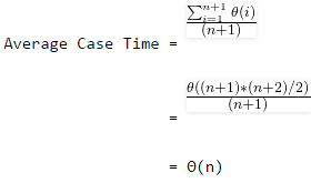
In average case analysis, we take all possible inputs and calculate computing time for all of the inputs. Sum all the calculated values and divide the sum by total number of inputs. We must know (or predict) distribution of cases. For the linear search problem, let us assume that all cases are uniformiy distributed (including the case of x not being present in array). So we sum all the cases and divide the sum by (n+1). Following is the value of average case time complexity.
Best Case Analysis (Bogus)
In the best case analysis, we calculate lower bound on running time of an algorithm. We must know the case that causes minimum number of operations to be executed. In the linear search problem, the best case occurs when x is present at the first location. The number of operations in the best case is constant (not dependent on n). So time complexity in the best case would be Θ(1)
Most of the times, we do worst case analysis to analyze algorithms. In the worst analysis, we guarantee an upper bound on the running time of an algorithm which is good information.
The average case analysis is not easy to do in most of the practical cases and it is rarely done. In the average case analysis, we must know (or predict) the mathematical distribution of all possible inputs.
The Best Case analysis is bogus. Guaranteeing a lower bound on an algorithm doesn’t provide any information as in the worst case, an algorithm may take years to run.
For some algorithms, all the cases are asymptotically same, i.e., there are no worst and best cases. For example, Merge Sort. Merge Sort does Θ(nLogn) operations in all cases. Most of the other sorting algorithms have worst and best cases. For example, in the typical implementation of Quick Sort (where pivot is chosen as a corner element), the worst occurs when the input array is already sorted and the best occur when the pivot elements always divide array in two halves. For insertion sort, the worst case occurs when the array is reverse sorted and the best case occurs when the array is sorted in the same order as output.
Analysis of Algorithms | (Asymptotic Notations)
We have discussed Asmptotic Analysis, and Worst, Average and Best Cases of Algorithms. The main idea of asymptotic analysis is to have a measure of efficiency of algorithms that doesn’t depend on machine specific constants, and doesn’t require algorithms to be implemented and time taken by programs to be compared. Asymptotic notations are mathematical tools to represent time complexity of algorithms for asymptotic analysis. The following 3 asymptotic notations are mostly used to represent time complexity of algorithms.
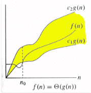
1) Θ Notation: The theta notation bounds a functions from above and below, so it defines exact asymptotic behavior.
A simple way to get Theta notation of an expression is to drop low order terms and ignore leading constants. For example, consider the following expression.
3n3 + 6n2 + 6000 = Θ(n3)
Dropping lower order terms is always fine because there will always be a n0 after which Θ(n3) has higher values than Θn2) irrespective of the constants involved.
For a given function g(n), we denote Θ(g(n)) is following set of functions.
Θ(g(n)) = {f(n): there exist positive constants c1, c2 and n0 such
that 0 <= c1*g(n) <= f(n) <= c2*g(n) for all n >= n0}
The above definition means, if f(n) is theta of g(n), then the value f(n) is always between c1*g(n) and c2*g(n) for large values of n (n >= n0). The definition of theta also requires that f(n) must be non-negative for values of n greater than n0.
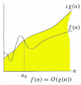
2) Big O Notation: The Big O notation defines an upper bound of an algorithm, it bounds a function only from above. For example, consider the case of Insertion Sort. It takes linear time in best case and quadratic time in worst case. We can safely say that the time complexity of Insertion sort is O(n^2). Note that O(n^2) also covers linear time.
If we use Θ notation to represent time complexity of Insertion sort, we have to use two statements for best and worst cases:
1. The worst case time complexity of Insertion Sort is Θ(n^2).
2. The best case time complexity of Insertion Sort is Θ(n).
The Big O notation is useful when we only have upper bound on time complexity of an algorithm. Many times we easily find an upper bound by simply looking at the algorithm.
O(g(n)) = { f(n): there exist positive constants c and
n0 such that 0 <= f(n) <= cg(n) for
all n >= n0}
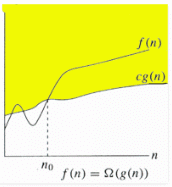
3) Ω Notation: Just as Big O notation provides an asymptotic upper bound on a function, Ω notation provides an asymptotic lower bound.
Ω Notation< can be useful when we have lower bound on time complexity of an algorithm. As discussed in the previous post, the best case performance of an algorthm is generally not usefull, the Omega notation is the least used notation among all three.
For a given function g(n), we denote by Ω(g(n)) the set of functions.
Ω (g(n)) = {f(n): there exist positive constants c and
n0 such that 0 <= cg(n) <= f(n) for
all n >= n0}.
Let us consider the same Insertion sort example here. The time complexity of Insertion Sort can be written as Ω(n), but it is not a very useful information about insertion sort, as we are generally interested in worst case and sometimes in average case.
Exercise:
Which of the following statements is/are valid?
1. Time Complexity of QuickSort is Θ(n^2)
2. Time Complexity of QuickSort is O(n^2)
3. For any two functions f(n) and g(n), we have f(n) = Θ(g(n)) if and only if f(n) = O(g(n)) and f(n) = Ω(g(n)).
4. Time complexity of all computer algorithms can be written as Ω(1)
Analysis of Algorithms | (Analysis of Loops)
We have discussed Asymptotic Analysis, Worst, Average and Best Casees and Asymptotic Notations in previous posts. In this post, analysis of iterative programs with simple examples is discussed.
1) O(1): Time complexity of a function (or set of statements) is considered as O(1) if it doesn’t contain loop, recursion and call to any other non-constant time function.
// set of non-recursive and non-loop statements
For example swap() function has O(1) time complexity.
A loop or recursion that runs a constant number of times is also considered as O(1). For example the following loop is O(1).
// Here c is a constant
for (int i = 1; i <= c; i++) {
// some O(1) expressions
}
2) O(n): Time Complexity of a loop is considered as O(n) if the loop variables is incremented / decremented by a constant amount. For example following functions have O(n) time complexity.
// Here c is a positive integer constant
for (int i = 1; i <= n; i += c) {
// some O(1) expressions
}
for (int i = n; i > 0; i -= c) {
// some O(1) expressions
}
3) O(nc): Time complexity of nested loops is equal to the number of times the innermost statement is executed. For example the following sample loops have O(n2) time complexity
for (int i = 1; i <=n; i += c) {
for (int j = 1; j <=n; j += c) {
// some O(1) expressions
}
}
for (int i = n; i > 0; i += c) {
for (int j = i+1; j <=n; j += c) {
// some O(1) expressions
}
For example Selection sort and Insertion Sort have O(n2) time complexity.
4) O(Logn) Time Complexity of a loop is considered as O(Logn) if the loop variables is divided / multiplied by a constant amount.
for (int i = 1; i <=n; i *= c) {
// some O(1) expressions
}
for (int i = n; i > 0; i /= c) {
// some O(1) expressions
}
For example Binary Search(refer interative implementation) has O(Logn) time complexity.
5) O(LogLogn) Time Complexity of a loop is considered as O(LogLogn) if the loop variables is reduced / increased exponentially by a constant amount.
// Here c is a constant greater than 1
for (int i = 2; i <=n; i = pow(i, c)) {
// some O(1) expressions
}
//Here fun is sqrt or cuberoot or any other constant root
for (int i = n; i > 0; i = fun(i)) {
// some O(1) expressions
}
How to combine time complexities of consecutive loops?
When there are consecutive loops, we calculate time complexity as sum of time complexities of individual loops.
for (int i = 1; i <=m; i += c) {
// some O(1) expressions
}
for (int i = 1; i <=n; i += c) {
// some O(1) expressions
}
Time complexity of above code is O(m) + O(n) which is O(m+n)
If m == n, the time complexity becomes O(2n) which is O(n).
How to calculate time complexity when there are many if, else statements inside loops?
As discussed here, worst case time complexity is the most useful among best, average and worst. Therefore we need to consider worst case. We evaluate the situation when values in if-else conditions cause maximum number of statements to be executed.
For example consider the liner search function where we consider the case when element is present at the end or not present at all.
When the code is too complex to consider all if-else cases, we can get an upper bound by ignoring if else and other complex control statements.
How to calculate time complexity of recursive functions?
Time complexity of a recursive function can be written as a mathematical recurrence relation. To calculate time complexity, we must know how to solve recurrences. We will soon be discussing recurrence solving techniques as a separate post.
What does ‘Space Complexity’ mean?
Space Complexity:
The term Space Complexity is misused for Auxiliary Space at many places. Following are the correct definitions of Auxiliary Space and Space Complexity.
Auxiliary Space is the extra space or temporary space used by an algorithm.
Space Complexity of an algorithm is total space taken by the algorithm with respect to the input size. Space complexity includes both Auxiliary space and space used by input.
For example, if we want to compare standard sorting algorithms on the basis of space, then Auxiliary Space would be a better criteria than Space Complexity. Merge Sort uses O(n) auxiliary space, Insertion sort and Heap Sort use O(1) auxiliary space. Space complexity of all these sorting algorithms is O(n) though.
|
81 videos|113 docs|33 tests
|
FAQs on Asymptotic Worst Case Time & Space Complexity - Algorithms - Computer Science Engineering (CSE)
| 1. What is the meaning of asymptotic worst-case time complexity in computer science engineering? |  |
| 2. How is asymptotic worst-case space complexity different from time complexity in computer science engineering? | |
| 3. Why is it important to analyze the asymptotic worst-case time complexity of an algorithm? | |
| 4. How can the asymptotic worst-case time complexity of an algorithm be represented? | |
| 5. Can the asymptotic worst-case time complexity of an algorithm change for different inputs? | |


Exam
,Asymptotic Worst Case Time & Space Complexity | Algorithms - Computer Science Engineering (CSE)
,Previous Year Questions with Solutions
,Semester Notes
,shortcuts and tricks
,Viva Questions
,Asymptotic Worst Case Time & Space Complexity | Algorithms - Computer Science Engineering (CSE)
,Important questions
,Summary
,MCQs
,practice quizzes
,study material
,Asymptotic Worst Case Time & Space Complexity | Algorithms - Computer Science Engineering (CSE)
,Objective type Questions
,ppt
,Free
,Extra Questions
,Sample Paper
,past year papers
,video lectures
,mock tests for examination
;


Asymptotic Worst Case Time & Space Complexity Free PDF Download
Importance of Asymptotic Worst Case Time & Space Complexity
Asymptotic Worst Case Time & Space Complexity Notes
Asymptotic Worst Case Time & Space Complexity Computer Science Engineering (CSE) Questions
Study Asymptotic Worst Case Time & Space Complexity on the App
|
© EduRev
|
Education Revolution
|


|


