Distribution System

Introduction to Distribution System
- Main canal
- Branch canal
- Distributaries
- Minors
- Water courses
Basic terms and definitions
Gross Commanded Area (GCA): The total area lying within the boundary of an irrigation project that can be economically commanded without regard to the limitation of available water. It includes both cultivable and non-cultivable lands.
Culturable Commanded Area (CCA): The part of the GCA on which cultivation is possible; sometimes also called net commanded area before taking cropping intensity into account.
Intensity of irrigation: The ratio of the area actually irrigated during a crop season to the net CCA, usually expressed as a percentage.
Annual irrigation intensity: The ratio of the total area irrigated during the whole year (sum over all crops and seasons) to the CCA, usually expressed as a percentage.
Time factor: The ratio of the number of days the canal actually has to run to the base period (in days) for which irrigation is planned.
Capacity factor: The ratio of the mean supply discharge actually available to the full supply discharge (design capacity) of the canal.
Shear stress (average unit tractive force) of a canal bed: The average tractive force per unit area acting on the bed is given by the product of unit weight of water, hydraulic mean depth and bed slope. In symbolic form:
τ = γw R S
Where τ is unit tractive force, γw is the unit weight of water, R is the hydraulic mean depth and S is the bed slope. (Take care of consistent units when evaluating τ.)
Hydraulic formulae for open channels
Several empirical and semi-empirical formulae are used for estimating mean velocity and discharge in open channels. The commonly used relations are Manning's formula, Chezy's formula (and Strickler/Strickler-type relations), Kutter's formula and others. These formulae relate mean velocity, hydraulic radius, slope and channel roughness.
Manning's formula

Manning's formula gives the mean velocity in uniform flow as a function of hydraulic radius and bed slope. In the usual functional form:
V = (1/n) R^(2/3) S^(1/2)
Where V is mean velocity, n is Manning's roughness coefficient, R is hydraulic radius and S is energy or bed slope. Discharge Q is obtained as Q = A·V, where A is the area of flow.
Chezy's (and Strickler/Strickler-type) relation

Chezy's formula expresses mean velocity as:
V = C √(R S)
Where C is the Chezy coefficient which depends on channel roughness and hydraulic radius. Strickler (often spelled Strickler or Strickler/Stickler in some texts) proposed expressions to estimate C from roughness characteristics and hydraulic radius; such expressions make Chezy's formula usable with a roughness parameter.
Kutter's formula
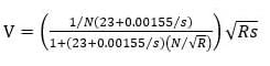
Kutter's formula gives an empirical relationship for the Chezy coefficient or for velocity that accounts for channel roughness and hydraulic radius. It is widely used in practice where roughness characteristics and side slopes require a refined estimate of the velocity coefficient.
Regime theories for alluvial channels
Alluvial channels carry sediment and are subject to both deposition (silting) and erosion (scouring). Several classical theories describe the conditions under which a channel can be approximately in equilibrium (no net silting or scouring) and provide design guidance for stable channel sections.
Kennedy's silt theory
Kennedy's investigations: R. G. Kennedy studied canal systems and proposed a silt theory based on the idea that sediment particles remain in suspension by vertical eddy currents generated by flow turbulence. The upward component of eddies tends to lift particles while gravity causes them to settle. If the flow velocity is sufficient to create eddies that keep particles just in suspension, there will be neither net silting nor scouring.
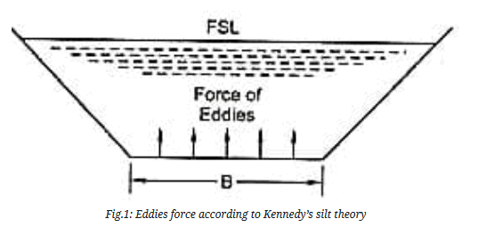
Critical velocity based on Kennedy's silt theory: The critical velocity is the mean velocity required to keep the channel free from net silting or scouring. It is expressed as a function of the full supply depth D in the form:

Where V0 is the critical velocity and D is the full supply depth. The empirical constants in the relationship are:
- C = 0.546
- n = 0.64
Thus the critical velocity may be obtained from the depth using the above empirical expression. Use consistent units when applying the formula.
Lacey's regime theory
Philosophy: Lacey studied stable river channels and developed formulae (now commonly known as Lacey's regime relations) for designing canals in alluvial soils. He pointed out that a channel might not be in a regime condition even if it exhibits neither silting nor scouring for short periods, and he distinguished three regime conditions.
Types of regime according to Lacey:
- True regime: A channel is in true regime when water and sediment are transported in equilibrium so that there is neither silting nor scouring. Lacey further stated that for true regime the following conditions should be approximately satisfied: discharge should be steady; the channel should flow through incoherent alluvium that can be scoured or deposited freely; the silt grade should be constant; and the silt charge (minimum transported load) should be constant. In practice these ideal conditions are rarely fully satisfied.
- Initial regime: When only the bed slope varies while the cross-section or wetted perimeter remains essentially unchanged, the channel may show non-siltation and non-scouring behaviour and is said to be in initial regime.
- Final regime: When both bed and sides are free to adjust, and all variables (perimeter, depth, slope etc.) reach an equilibrium for the given discharge and silt grade, the channel attains a final or permanent stability called final regime.
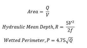
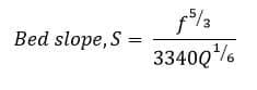
Lacey's design procedure (conceptual steps):
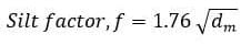
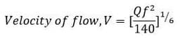
- Obtain the canal discharge Q and the mean particle size dm of the transported sediment.
- Compute the silt factor from the mean particle diameter using Lacey's empirical relation. (Formula appears as an image below.)
- Using the discharge and silt factor, compute the design velocity V from Lacey's empirical velocity relation. (Formula appears as an image below.)
- Find the flow area A from A = Q / V. Determine the mean hydraulic depth R and wetted perimeter P corresponding to the chosen section shape.
- Determine the bed slope S required to sustain the regime by substituting the silt factor and discharge in Lacey's slope relation. (Formula appears as an image below.)
For the actual algebraic expressions used in Lacey's method, see the images placed below in the same order as the procedural steps.
Drawbacks and limitations of Lacey's silt theory
- Lacey did not fully explain the mechanical properties that govern the behaviour of alluvial channels.
- Flow velocity varies between bed and sides; Lacey used a single silt factor although two differing factors would be more realistic.
- The semi-elliptical cross-section proposed by Lacey as the ideal channel shape is not universally convincing or economical.
- Silt concentration in the flow is not explicitly accounted for in Lacey's equations.
- Attrition (breakage and rounding) of silt particles during transport is ignored.
- Definitions for silt grade and silt charge are not always precise in Lacey's original formulation.
Design steps and practical remarks for distribution systems
Design of canal distribution systems follows a hierarchy: determine the project command area, compute water duty and required supply, design main canal and branch canal sections, and then design distributaries, minors and field channels (water courses) to deliver water to the fields with suitable time and capacity factors.
- Estimate crop water requirements for the command (seasonal and annual) and derive the design duty and discharge requirements.
- Select suitable channel section shapes (trapezoidal, semi-elliptical, etc.) considering economy, ease of maintenance and hydraulic stability. For alluvial channels, regime theories (Lacey, Kennedy) may guide section proportions.
- Choose appropriate hydraulic formula (Manning, Chezy with Strickler/Kutter) depending on available data for roughness and hydraulic radius; compute required bed slope or provide design roughness to meet desired velocity.
- Check tractive forces against permissible bed shear stress of bed material to avoid excessive scouring or deposition; where necessary, provide protection (revetment, lining) or grading measures.
- Ensure distributary and minor layouts give equitable, economic conveyance with appropriate outlets, head regulators and measurement devices to control diversion and measure supplies.
- Consider operational factors (time factor, capacity factor, canal operation schedules, maintenance access, sediment removal arrangements) when finalising dimensions and layout.
Practical example (illustrative, symbolic)
To illustrate the relation between discharge, channel area and velocity without numerical computation:
If the canal discharge is Q, and the design velocity (from Manning's or Lacey's relation) is determined as V, then the required wetted area of flow is
A = Q / V
Once A is fixed, choose a practical section shape and depth so that the hydraulic radius R and wetted perimeter are consistent. Use the chosen hydraulic formula to check that the computed velocity at that section and slope equals the design velocity.
Summary
Distribution systems consist of main canals, branch canals, distributaries, minors and water courses. Core design concepts include estimating commanded areas and irrigation intensities, computing supply requirements, and selecting channel sections and slopes using hydraulic formulae (Manning, Chezy/Kutter, etc.) and regime theories (Kennedy and Lacey). Each theory has assumptions and limitations; practical design combines hydraulic calculations with geotechnical and operational considerations to arrive at stable, economical and serviceable canal systems.
FAQs on Distribution System
| 1. What is a distribution system in supply chain management? |  |
| 2. What are the key components of a distribution system? | |
| 3. How does a distribution system benefit businesses? | |
| 4. What challenges are faced in managing a distribution system? | |
| 5. How can technology help in optimizing a distribution system? | |