Transfer Function | Control Systems - Electrical Engineering (EE) PDF Download

Introduction
The Transfer Function (TF) of a system, denoted , is defined as the ratio of the output to the input in the Laplace domain, assuming zero initial conditions and equilibrium.
Mathematically:
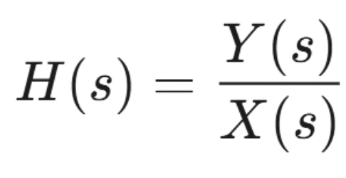
Here, represents the Laplace transform of the input, and represents the Laplace transform of the output.
Impulse Response
Since we know that in the time domain, generally, we define the input to a system as x(t), and the output of the system as y(t). The relationship between the input and the output is represented as the impulse response, h(t).
We can use the following equation to define the impulse response:
h(t) = y(t) / x(t)
- The Impulse Function, denoted with δ(t) is a function defined piece-wise as follows
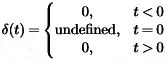
- An examination of the impulse function shows that it is related to the unit-step function as follows
u(t) = ∫δ(t) or δ(t) = du(t) / dt - The impulse response (IR) must always satisfy the following condition, or else it is not a true impulse function

Convolution in Time Domain
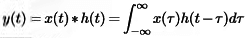
If we have the system input and the impulse response of the system, we can calculate the system output using the convolution operation as such as
y(t) = h(t) ∗ x(t).
Time-Invariant System Response
- If the system is time-invariant, then the general description of the system can be replaced by a convolution integral of the system's impulse response and the system input. We can call this the convolution description of a system.
Methods of Obtaining a Transfer Function
There are major two ways of obtaining a transfer function for the control system. The ways are:
- Block Diagram Method: It is not convenient to derive a complete transfer function for a complex control system. Therefore the transfer function of each element of a control system is represented by a block diagram. Block diagram reduction techniques are applied to obtain the desired transfer function.
- Signal Flow Graphs: The modified form of a block diagram is a signal flow graph. Block diagrams visually outline a control system, while signal flow graphs provide a more compact representation.
Poles and Zeros of Transfer Function
Generally, a function can be represented to its polynomial form. For example, Now similarly transfer function of a control system can also be represented as
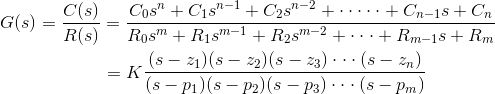
Where K is known as the gain factor of the transfer function.
Now in the above function if s = z1, or s = z2, or s = z3,….s = zn, the value of transfer function becomes zero. These z1, z2, z3,….zn, are roots of the numerator polynomial. As for these roots the numerator polynomial, the transfer function becomes zero, these roots are called zeros of the transfer function.
Now, if s = p1, or s = p2, or s = p3,….s = pm, the value of transfer function becomes infinite. Thus the roots of denominator are called the poles of the function.
Let’s represent the transfer function in its polynomial form: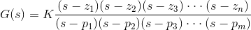
Now, let us consider s approaches to infinity as the roots are all finite number, they can be ignored compared to the infinite s. Therefore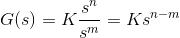 Hence, when s → ∞ and n > m, the function will have also value of infinity, that means the transfer function has poles at infinite s, and the multiplicity or order of such pole is n – m. Again, when s → ∞ and n < m, the transfer function will have value of zero that means the transfer function has zeros at infinite s, and the multiplicity or order of such zeros is m – n.
Convolution Theorem
- Convolution in the time domain turns into multiplication in the complex Laplace domain.
- Multiplication in the time domain turns into convolution in the complex Laplace domain.
L[f(t) ∗ g(t)] = F(s)G(s)
L[f(t)g(t)] = F(s) ∗ G(s)
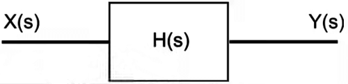
Result: If the complex Laplace variable is s, then we generally denote the transfer function of a system as either G(s) or H(s). If the system input is X(s), and the system output is Y(s), then the transfer function can be defined as such
H(s) = Y(s)/X(s) - So if we know the input to a given system, and we have the transfer function of the system, we can solve for the system output by multiplying as
Y(s) = H(s)X(s)
Example: Impulse Response
- Since we know that the Laplace transform of the impulse function, δ(t) is L[δ(t)] = 1
- So, when we put this into the relationship between the input, output, and transfer function, we get
Y(s) = X(s)H(s)
or Y(s) = (1)H(s)
or Y(s) = H(s)
In other words, the "impulse response" is the o/p of the system when we input an impulse function.
Transfer Functions for Linear Systems
Consider a linear input/output system described by the controlled differential equation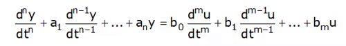
where u is the input and y are the output.
- To obtain the transfer function of the system of last equation let us input be u(t) = est.
- Since the system is linear, there is an output of the system that is also an exponential function ⇒ y(t) = Yoest.
- Inserting the signals into last equation ,we find
(sn + a1sn−1 +···+ an)yo.est = (bosm + b1sm−1···+ bm)e−st - And the response of the system can be completely described as
a(s) = sn + a1sn−1 +···+ an & b(s) = bosm + b1sm−1 + ···+ bm
y(t) = y0est = (b(s) / a(s))est - So the transfer function of the given function is given by
G(s) = b(s) / a(s)
Transfer Function Alternative Method
To investigate how a linear system responds to the exponential input u(t) = est we consider the state space system
dx/dt = Ax + Bu
y = Cx + Du
Let the input signal be u(t) = est and assume that s ≠ λi(A), where i = 1,...,n, where λi(A) is the ith eigenvalue of A. then
Since s ≠ λ(A) the integral can be evaluated and we get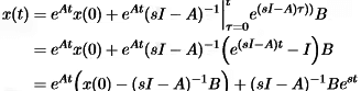
& Output y(t) = Cx(t) + Du(t)
= CeAt{x(0) − (sI − A)−1B} + [D + C(sI − A)−1B]est
Note: One term of the output is proportional to the input u(t) = est. This term is called the pure exponential response.
- If the initial state is chosen as x(0) = (sI −A)−1B
- the output only consists of the only exponential response and both the state and the output are directly proportional to the input
x(t) = (sI − A)−1Best = (sI − A)−1Bu(t)
y(t) = [C(sI − A)−1B+D]est = [C(sI − A)−1B + D]u(t). - The ratio of the output and the input
G(s) = C(sI − A)−1B + D is the transfer function of the system. - For Homogeneous Equation i.e; D = 0 then
G(s) = C(sI − A)−1B is the transfer function of the system.
The Concept of Pole & Zero
- Poles and Zeros of a transfer function are the frequencies for which the value of the transfer function becomes infinity or zero respectively.
- The transfer function has many useful explanations and the features of a transfer function are often associated with important system properties. Three of the most important features are the gain and the locations of the poles and zeros.
H(s) = N(s)/D(s) - In the above equation, N(s) and D(s) are simple polynomials in s. Zeros are the roots of N(s) by setting N(s) = 0 and solving for s. Poles are the roots of D(s), by setting D(s) = 0 and solving for s.
- In general Transfer Function must not have more zeros than poles, we can state that the polynomial order of D(s) must be greater than or equal to the polynomial order of N(s).
Effects of Poles and Zeros
- when s approaches a zero (Zeros of Transfer function), the numerator of the transfer function N(s)→0.
- When s approaches a pole (Poles of Transfer Function) the denominator of the transfer function D(s)→0 & the value of the transfer function approaches infinity.
- An output value of infinity should raise an alarm bell for people who are familiar with BIBO stability.
- Poles & Zeros of a transfer function are represented in S-Plane, In s-plane s = σ ± jω where σ represent the attenuation on X-axis & ω represents the angular velocity represented on the y-axis.
- In s-plane, the Poles are located by a cross (*) & the Zeros are located by dot (.)
- For a Stable System, All the Poles & Zeros of a Transfer Function must be lie in the left half of s-plane.
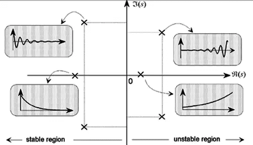
Note: If the Poles or Zero lie on the imaginary axis then it must be simple (order only 1) then the system is said to be Marginally Stable, If the Order of multiplicity of Poles or Zeros on Imaginary Axis is more than 1 in that case system will become Unstable.
Example
The transfer function of the system, G(s) = I(s)/V(s), the ratio of output to input.
1) Let us explain the concept of poles and zeros of transfer function through an example.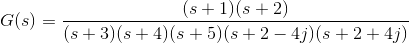 Solution
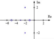
The zeros of the function are, -1, -2 and the poles of the functions are -3, -4, -5, -2 + 4j, -2 – 4j.
Here n = 2 and m = 5, as n < m and m – n = 3, the function will have 3 zeros at s → ∞. The poles and zeros are plotted in the figure below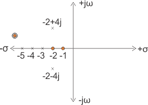 2) Let us take another example of transfer function of control system
 Solution
In the above transfer function, if the value of numerator is zero, then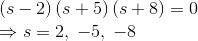 These are the location of zeros of the function.
Similarly, in the above transfer function, if the value of denominator is zero, then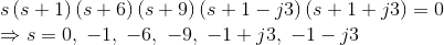 These are the location of poles of the function.
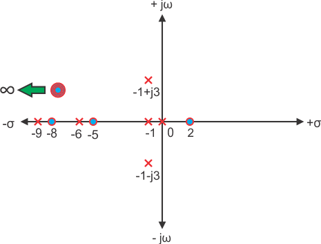 As the number of zeros should be equal to number of poles, the remaining three zeros are located at s →∞.
Example of Transfer Function of a Network
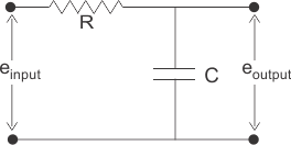
3.)Solution
In the above network it is obvious that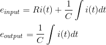 Let us assume,
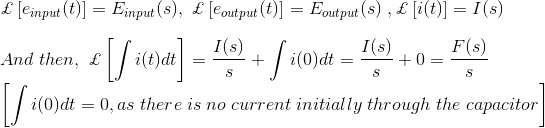 Taking the Laplace transform of above equations with considering the initial condition as zero, we get,
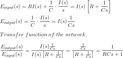
Transfer Function of Closed Loop System
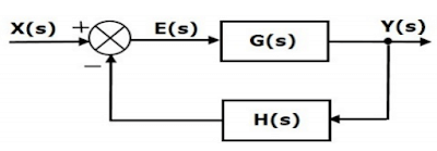 Block diagram of Closed Loop SystemE(s) = Actuating or Error Signal
X(s) = Reference Input Signal.
G(s) = Forward Path Transfer Function.
Y(s) = Output Signal.
H(s) = Feedback Transfer Function.
B(s) = Feedback Signal.
So, the transfer function of the closed loop system is Y(s)/X(s).
From the block diagram,
Y(s) = G(s).E(s) .........1
B(s) = H(s).Y(s) .........2
E(s) = X(s) + B(s) .........3a (For positive feedback)
= X(s) - B(s) ..........3b (For negative feedback)
For Negative Feedback (using eq.3b)
Put the value of E(s) from eq.3b in eq.1Y(s) = G(s).[X(s)-B(s)]
Y(s) = G(s).X(s) - G(s).B(s) .........4
Put the value of B(s) from eq.2 in eq.4
Y(s) = G(s).X(s) - G(s).H(s).Y(s)
Y(s) + G(s).H(s).Y(s) = G(s).X(s)
Y(s){1 + G(s).H(s)} = G(s).X(s)
Y(s)/X(s) = G(s) / {1 +G(s).H(s)} .........5
For Positive Feedback (using eq. 3a)
For positive feedback system we will use eq.3a and repeat the all the same steps and we will get the transfer function as:
Y(s)/X(s) = G(s) / {1 - G(s).H(s)} .........6
For Unity Feedback
For unity feedback H(s) = 1, the eq.5 & eq.6 will become
Y(s)/X(s) = G(s)/{1 + G(s)} .......for negative unity feedback
Y(s)/X(s) = G(s)/{1 - G(s)} ........for positive unity feedback
Frequency Response
Frequency response describes a system’s steady-state behavior when driven by sinusoidal inputs of varying frequencies. It is derived from the transfer function by evaluating it at s=jω, where ω is the angular frequency, revealing how the system modifies the amplitude and phase of these inputs.
- Definition: The frequency response is the complex function obtained from the transfer function G(s) at s=jω. It quantifies the system’s gain (amplitude change) and phase shift for sinusoidal inputs, assuming a linear time-invariant (LTI) system.
- Relation to Transfer Function: Poles and zeros of G(s) shape the frequency response. Poles near the imaginary axis amplify specific frequencies (resonance), while zeros cause attenuation or phase shifts.
- Significance: Frequency response is crucial for analyzing system performance, including bandwidth (range of frequencies processed) and stability margins (gain and phase margins). It guides controller design to meet performance goals.
- Visualization: Bode plots, showing magnitude and phase versus frequency, provide a theoretical tool to study frequency response and assess system behavior.
- Limitations: It focuses on steady-state behavior and LTI systems, less suited for transient analysis or nonlinear systems.
Closed-Loop Systems
Sensitivity analysis examines how changes in system parameters or external disturbances affect performance. In closed-loop systems, feedback reduces sensitivity, enhancing robustness against uncertainties.- Definition: Sensitivity measures how variations in parameters (e.g., gain) alter the system’s transfer function. Low sensitivity ensures consistent performance despite uncertainties.
- Role of Feedback: Negative feedback reduces sensitivity by making the closed-loop transfer function less dependent on forward-path parameters. It also mitigates external disturbances (disturbance rejection).
- Trade-Offs: While feedback improves robustness, high feedback gain may compromise stability or limit bandwidth, requiring careful design.
- Significance: Sensitivity analysis is vital for designing reliable control systems, ensuring performance in applications with variable conditions (e.g., manufacturing, aerospace).
- Limitations: It assumes small parameter changes and linear systems, less applicable to large variations or nonlinear dynamics.
|
53 videos|115 docs|40 tests
|
FAQs on Transfer Function - Control Systems - Electrical Engineering (EE)
| 1. What is the Convolution Theorem in the context of transfer functions for linear systems? |  |
| 2. What are Poles and Zeros in the concept of transfer functions for linear systems? | |
| 3. How can the transfer function of a closed-loop system be determined in electrical engineering? | |
| 4. How do transfer functions play a crucial role in analyzing and designing linear systems in electrical engineering? | |
| 5. What is the significance of the Convolution Theorem in signal processing and control systems design? | |


ppt
,Extra Questions
,Transfer Function | Control Systems - Electrical Engineering (EE)
,Transfer Function | Control Systems - Electrical Engineering (EE)
,past year papers
,Summary
,Sample Paper
,Viva Questions
,video lectures
,practice quizzes
,Free
,study material
,Important questions
,Transfer Function | Control Systems - Electrical Engineering (EE)
,mock tests for examination
,shortcuts and tricks
,Previous Year Questions with Solutions
,Semester Notes
,Exam
,MCQs
,Objective type Questions
;


Transfer Function Free PDF Download
Importance of Transfer Function
Transfer Function Notes
Transfer Function Electrical Engineering (EE) Questions
Study Transfer Function on the App
|
© EduRev
|
Education Revolution
|


|


