Working in Excel | Computer Science - Class 5 PDF Download
Introduction:-
Excel is a spreadsheet program that allows you to store, organize and analyze information, in this unit, you will learn about the MS-Excel 2007 environment.
The Excel Interface:-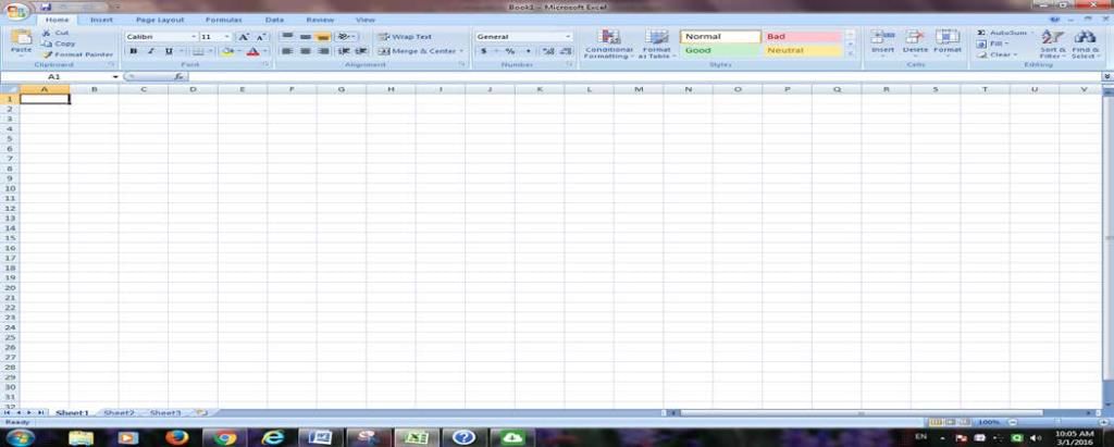
Fig: Excel Sheet
3.1 Working with Sheets:-
What is worksheet/sheet: - A worksheet is a collection of cells where you keep and manipulate the data. By default, each Excel workbook contains three worksheets.
3.1.1 Creating/Deleting Sheets:-
When you open Excel, Excel automatically selects Sheet1 for you. The name of the worksheet appears on its sheet tab at the bottom of the document window.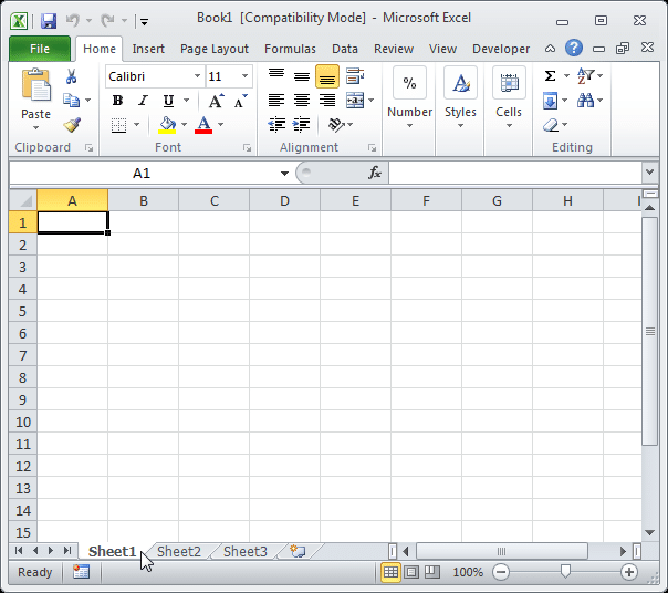
Fig: Creating or Deleting Sheet
To select one of the other two worksheets, simply click on the sheet tab of Sheet2 or Sheet3.
Insert a Worksheet
You can insert as many worksheets as you want. To quickly insert a new worksheet, click the Insert Worksheet tab at the bottom of the document window.
Result:
Delete a Worksheet
To delete a worksheet, right click on a sheet tab and choose Delete.
1. For example, delete Sheet4, Sheet2 and Sheet3.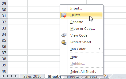 Result:
3.1.2 Renaming Sheets:-
By default, the worksheets are named Sheet1, Sheet2 and Sheet3. To give a worksheet a more specific name, execute the following steps.
1. Right click on the sheet tab of Sheet1.
2. Choose Rename.
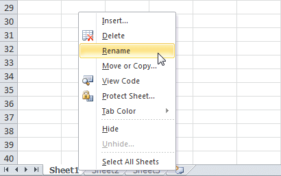
3. For example, type Sales 2010.
3.1.3 Copying / Moving Sheets:-
Copy a Worksheet
Imagine, you have got the sales for 2010 ready and want to create the exact same sheet for 2011, but with different data. You can recreate the worksheet, but this is time-consuming. It's a lot easier to copy the entire worksheet and only change the numbers.
1. Right click on the sheet tab of Sales 2010.
2. Choose Move or Copy...
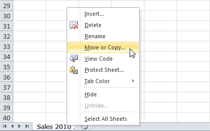 The 'Move or Copy' dialog box appears.
3. Select (move to end) and check Create a copy.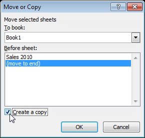
4. Click OK.
Result:
Note: you can even copy a worksheet to another Excel workbook by selecting the specific workbook from the drop-down list (see the dialog box shown earlier).
Move a Worksheet
To move a worksheet, click on the sheet tab of the worksheet you want to move and drag it into the new position.
1. For example, click on the sheet tab of Sheet4 and drag it before Sheet2.
Result:
3.2 Inserting New Row and Column:-
Insert Row, Column
To insert a row between the values 20 and 40 below, execute the following steps.
1. Select row 3.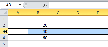
2. Right click, and then click Insert.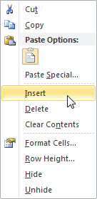
Result: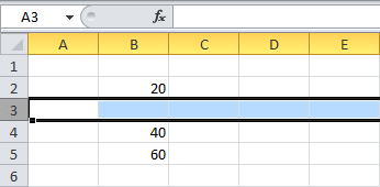 Note: - You can perform the same operation for inserting column.
3.3 Deleting/Hiding the Rows and Columns:-
Deleting the Rows and Columns:-
To delete a row between the values 20 and 40 below, execute the following steps.
1. Select row 3. 2. Right click, and then click delete.
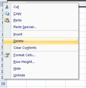 Result:
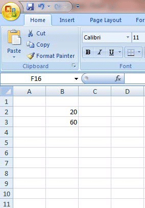
Hiding the Rows and Columns:-
To hide a row between the values 20 and 40 below, execute the following steps.
1. Select row 3. 2. Right click, and then click Hide.
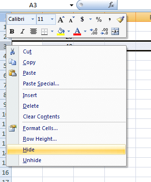
3. Result: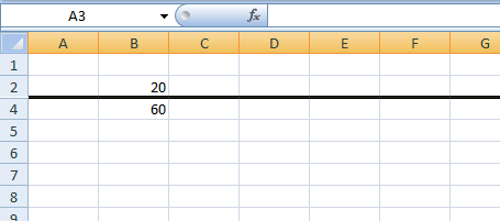
3.4 Changing the width and height of the column and row:-
On a worksheet, you can specify a column width of 0 (zero) to 255. This value represents the number of characters that can be displayed in a cell that is formatted with the standard font. The default column width is 8.43 characters. If a column has a width of 0 (zero), the column is hidden.
You can specify a row height of 0 (zero) to 409. This value represents the height measurement in points (1 point equals approximately 1/72 inch or 0.035 cm). The default row height is 12.75 points (approximately 1/6 inch or 0.4 cm). If a row has a height of 0 (zero), the row is hidden.
Set a column to a specific width
1. Select the column or columns that you want to change.
2. On the Home tab, in the Cells group, click Format.
3. Under Cell Size, click Column Width.
4. In the Column width box, type the value that you want.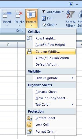
Set a row to a specific height
1. Select the row or rows that you want to change.
2. On the Home tab, in the Cells group, click Format.
3. Under Cell Size, click Row Height.
4. In the Row height box, type the value that you want.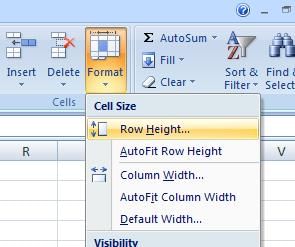
3.5 Find and Select the data in a given range.-
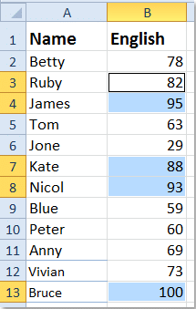
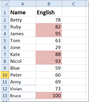
Supposing you have a data range as following screenshot, and now you want to find or select cells based on certain criteria information in Excel, for example, you will find or select the cells which contain the numbers between 80 and 100. How could you quickly solve this task?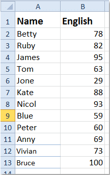

You can solve this task by following methods:-
(i) Filter cells based on certain criteria with Filter function
(ii) Find cells based on certain criteria with Conditional Formatting
(i) Filter cells based on certain criteria with Filter function
With Filter function of Excel, you can display the cell rows that you need and hide the unwanted rows. You can finish it with the following steps:
1. Highlight the column that you want to select the certain cells.
2. Click Data > Filter, see screenshot: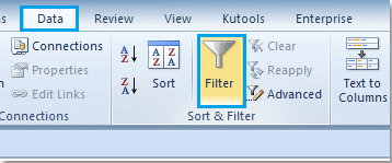
3. And a small triangle will display at the bottom right corner of the title, click the small triangle, and a menu will appear. Choose Number Filter > Custom Filter… See screenshot: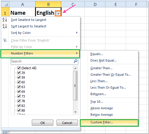
And a Custom AutoFilter dialog box will pop out. Then specify the criteria that you need as following screenshot: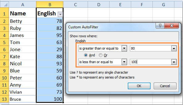
5. Click OK. And all of the cells which fit to the criteria have been displayed, and the others have been hidden.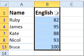 With this method, the other cells which don’t accord with the criteria will be hidden.
(ii) Find cells based on certain criteria with Conditional Formatting
Conditional Formatting utility can help you to find and format the cells which match your criteria in Excel, please do as this:
1. Select the data range that you want to use.
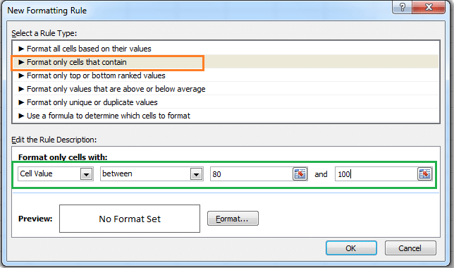
2. Click Home > Conditional Formatting > New Rule, see screenshot: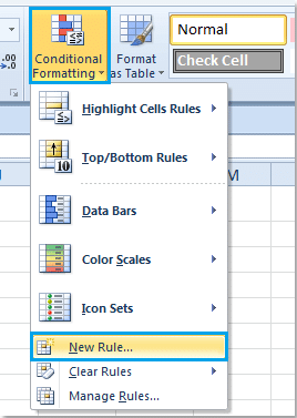 3. In the New Formatting Rule dialog box, select Format only cells that contain option under Select a Rule Type, and then specify the criteria you need under Format the Rule Description, see screenshot:
5. Then click Format button, in the Format Cells dialog, click Fill tab, and select one color you like to shade your cells. See screenshot: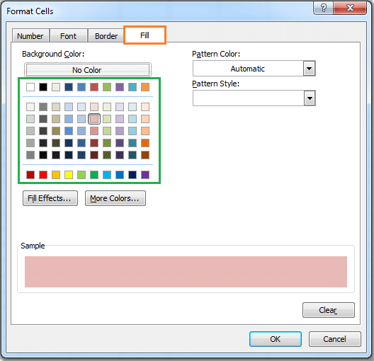 6. Click OK to close the dialogs, and the cells between 80 and 100 have been highlighted at once.
3.6 VIEW MENU
3.6.1 Gridlines:-
Gridlines are the faint lines that appear around cells in Excel 2007. They are used to distinguish cells on the worksheet.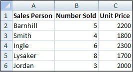 Note: - Gridlines do not print by default.
Show/Hide gridlines on a worksheet
(i) Hide gridlines on a worksheet:-
If the design of your workbook requires it, you can hide the gridlines: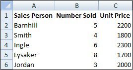 1. Select one or more worksheets.
2. On the View tab, in the Show/Hide group, clear the Gridlines check box. (ii) Show gridlines on a worksheet
If the gridlines on your worksheet are hidden, you can use the following procedure to show them again.
1. Select one or more worksheets.
2. On the View tab, in the Show/Hide group, select the Gridlines check box.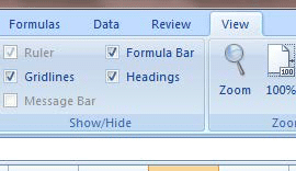 3.6.2 Freeze Panes
To keep an area of a worksheet visible while you scroll to another area of the worksheet, you can lock specific rows or columns in one area by freezing or splitting panes.
When you freeze panes, you keep specific rows or columns visible when you scroll in the worksheet. For example, you might want to keep row and column labels visible as you scroll.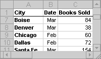
A solid line indicates that row 1 is frozen to keep column labels in place when you scroll.
Freeze panes to lock specific rows or columns:-
1. On the worksheet, do one of the following:
• To lock rows, select the row below the row or rows that you want to keep visible when you scroll.
• To lock columns, select the column to the right of the column or columns that you want to keep visible when you scroll.
To lock both rows and columns, click the cell below and to the right of the rows and columns that you want to keep visible when you scroll.
2. On the View tab, in the Window group, click the arrow below Freeze Panes.
3. Do one of the following:
• To lock one row only, click Freeze Top Row.
• To lock one column only, click Freeze First Column.
• To lock more than one row or column, or to lock both rows and columns at the same time, click Freeze Panes.
3.6.3 View side by side:-
You can quickly compare two worksheets in the same workbook or in different workbooks by viewing them side by side.
View two worksheets in the same workbook side by side
1. On the View tab, in the Window group, click New Window.
2. On the View tab, in the Window group, click View Side by Side .
3. In the workbook window, click the worksheets that you want to compare.
3.6.4 Synchronous Scrolling:-
If you want to compare the data simultaneously, throughout the Excel files. To do that, there is an option called Synchronous Scrolling, which is under View Side by Side. Just click Synchronous Scrolling. This option lets you scroll both files at the same time.
NOTE this option is available only when View Side by Side is turned on.
When you scroll, you will see both windows are scrolling at the same time so that comparing the two is quite simple.
|
36 videos|38 docs|27 tests
|
FAQs on Working in Excel - Computer Science - Class 5
| 1. What are the basic functions in Excel? |  |
| 2. How do I create a chart in Excel? |  |
| 3. How can I use conditional formatting in Excel? |  |
| 4. How do I create a pivot table in Excel? |  |
| 5. How can I protect cells or worksheets in Excel? |  |


