Variation of Flow Parameters in Time & Space - 1


Variation of Flow Parameters in Time and Space
Hydrodynamic parameters such as pressure, density and velocity may vary from one point to another in space and may also change with time at a fixed point. The character of these variations is used to classify flows into different types. The most common classifications are by steadiness and by uniformity.
Steady and Unsteady Flow
Steady Flow
Definition: A steady flow is one in which the hydrodynamic parameters and fluid properties at a given point do not change with time.
Using the Eulerian approach, where velocity and other field quantities are expressed as functions of space and time, a steady flow is described by the property that the partial derivative with respect to time at every fixed point is zero.
Implications:
- Velocity and acceleration are functions of space coordinates only (no explicit time dependence).
- The spatial distribution of hydrodynamic parameters is fixed in time; values may vary from point to point but this pattern does not change with time.
Using the Lagrangian approach (following individual fluid particles), time is inherent because particle motion is described as a function of time. In a steady flow, the velocities of all particles passing through a fixed point at different times are the same. Consequently, describing velocity for a single particle as it moves through space reproduces the same spatial velocity field given by the Eulerian representation; hence, for steady flow the Eulerian and Lagrangian descriptions are consistent with one another.
Unsteady Flow
Definition: An unsteady flow is one in which hydrodynamic parameters (for example, velocity, pressure, density) at a fixed point change with time.
Uniform and Non-uniform Flow
Uniform Flow
Definition: A uniform flow is one in which the velocity and other hydrodynamic parameters have the same value at every point of the flow field at a given instant.
In Eulerian notation, for a uniform flow the velocity is a function of time only (no spatial variation):

Implications:
- There is no spatial distribution of hydrodynamic parameters; the entire field has a unique value of each parameter at an instant.
- If the single value changes with time the flow is unsteady uniform. If that value does not change with time the flow is steady uniform.
- Therefore, steadiness and uniformity are independent properties: a flow can be steady but non-uniform, uniform but unsteady, both or neither.
Non-uniform Flow
Definition: A non-uniform flow is one in which velocity and/or other hydrodynamic parameters change from one spatial point to another.
Important points:
- Spatial changes may occur in the flow direction (streamwise variation) or in directions normal to the flow (cross-stream variation).
- Non-uniformity perpendicular to the flow is commonly found near solid boundaries because of viscosity, which reduces the relative fluid velocity to zero at the wall (the no-slip condition).
Four characteristic combinations
| Type | Example |
|---|---|
| 1. Steady uniform flow | Flow at constant rate through a duct of uniform cross-section (neglecting the thin boundary layer near walls) |
| 2. Steady non-uniform flow | Flow at constant rate through a duct of varying cross-section (for example, a tapering pipe) |
| 3. Unsteady uniform flow | Flow at varying rate through a long straight pipe of uniform cross-section (ignoring wall boundary layer) |
| 4. Unsteady non-uniform flow | Flow at varying rate through a duct of non-uniform cross-section |
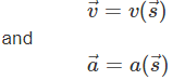
Material Derivative and Acceleration
To relate changes observed at a moving particle to changes observed at a fixed point, we introduce the material (or substantial) derivative. Consider a fluid particle whose position at time t is (x, y, z) in a Cartesian frame. Let the velocity components of the particle be u, v, w along x, y, z respectively. In Eulerian form these components are functions of space and time:
- u = u(x, y, z, t)
- v = v(x, y, z, t)
- w = w(x, y, z, t)
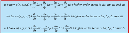
After an infinitesimal time Δt the particle moves to (x + Δx, y + Δy, z + Δz) and its velocity components change to u + Δu, v + Δv, w + Δw. Expanding the velocity increments by Taylor series gives the relation between the particle (material) rate of change and the local and convective changes:
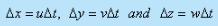
The spatial increments are related to the particle velocity components as:
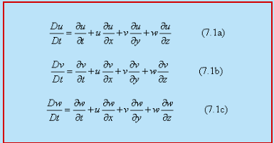
Substituting these expressions into the Taylor expansions produces the incremental form for Δu, Δv, Δw, and dividing by Δt and taking the limit Δt → 0 yields the material derivatives:


- In the limit Δt → 0 the equation becomes:

Material derivative (substantial derivative) operator
The operator for the total derivative following a fluid particle is:
The material derivative D/Dt relates to the partial derivative ∂/∂t as:
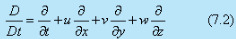
Explanation:
- The operator D/Dt is the material (substantial) derivative with respect to time; it represents the rate of change experienced by a specific fluid particle as it moves.
- The first term on the right hand side, ∂/∂t, is the local (temporal) derivative, which measures the rate of change at a fixed point in space.
- The remaining terms are the convective derivative terms and represent changes due to the particle moving through a spatially varying field.
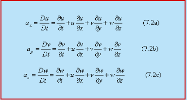
Thus the acceleration components (material accelerations) may be decomposed as:

or, in compact vector form:
Important points:
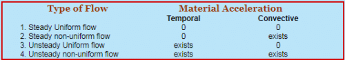
- In a steady flow the local (temporal) acceleration is zero because field values at fixed points are time-invariant.
- In a uniform flow the convective acceleration is zero because field values do not vary with space.
- In a flow that is both steady and uniform both local and convective accelerations vanish and the material acceleration is zero.
A compact table summarising which acceleration components exist for different flow types is shown below.
Acceleration in Cylindrical (Polar) Coordinates
For flows where cylindrical coordinates (r, θ, z) are convenient, velocity components and acceleration components acquire additional geometric terms. The velocity components are typically Vr, Vθ and Vz. The components of acceleration in r, θ and z directions are:
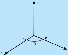
and explicitly:
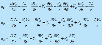
Explanation of additional terms:
- The term corresponding to -Vθ²/r (appearing as an inward radial acceleration) is the centripetal acceleration produced by change in direction of the azimuthal velocity.
- The term Vr Vθ / r represents a contribution to the azimuthal acceleration caused by variation of the radial velocity direction with θ.
Streamlines, Stream-tubes, Pathlines and Streaklines
Streamlines
Definition: A streamline is a curve which is everywhere tangent to the instantaneous velocity vector of the flow. It is a geometric representation of the velocity field at a given instant.
Using the Eulerian method, for a fixed instant of time a space curve drawn so that at every point it is tangent to the velocity vector is a streamline. For an unsteady flow the pattern of streamlines changes with time; for a steady flow the set of streamlines is fixed.
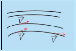
Alternative statement: The tangent to a streamline shows the direction of the instantaneous velocity at that point.
The differential equation of a streamline may be written as (velocity vector V and infinitesimal line element ds):

In Cartesian coordinates this reduces to the familiar form:

or, equivalently,

Stream-tube
Definition: A stream-tube is a bundle of neighbouring streamlines that form a passage through which fluid flows.
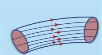
Properties:
- A stream-tube is bounded by streamlines; its lateral surface is formed by streamlines.
- No fluid crosses a streamline, therefore no fluid enters or leaves a stream-tube across its sides; fluid can enter or leave only through the ends of the tube.
- The whole flow field can be thought of as composed of many stream-tubes arranged in space.
Pathlines
Definition: A pathline is the actual trajectory traced by a single fluid particle as it moves through the flow. It follows the identity of that particle over time.
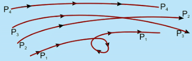
A family of pathlines represents trajectories of different particles (P1, P2, P3, ...). For steady flow, pathlines coincide with streamlines (because particle velocities at given points do not change with time).
Differences between Pathline and Streamline
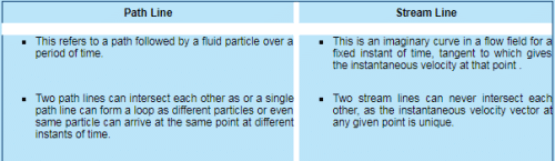
- Pathlines follow the motion of individual particles (Lagrangian viewpoint); streamlines are instantaneous direction lines of velocity at a fixed instant (Eulerian viewpoint).
- In general (unsteady flow) a pathline need not coincide with a streamline. In steady flow they coincide.
Streaklines
Definition: A streakline is the locus of all particles that have passed through a given fixed point in space. It is the line formed by fluid particles that have previously passed through the same location.
Features:
- A streakline is identified by a fixed spatial point (for example, a dye injector location); it is widely used in experimental flow visualisation.
- If dye is continuously injected at a fixed point, the observed dye pattern at a later time is a streakline.
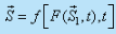
The equation of a streakline at time t may be derived by the Lagrangian description. If a particle passes through a fixed point at time τ and its position at later time t is given by the Lagrangian map, then collecting positions of all particles that passed through the fixed point for all τ up to t yields the streakline.


Solving for the parametric history of particles gives the streakline equation:

Substituting appropriate Lagrangian relations yields the final form:
Difference between Streakline and Pathline
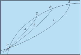
Qualitative description:
- Consider a fixed point P in the flow through which different particles pass at different times. In an unsteady flow particles arriving at P at different times follow different trajectories (pathlines) such as PAQ, PBR, PCS.
- At a chosen instant, the end points of these individual trajectories will be Q, R, S; joining S, R, Q and the injection point P gives the streakline at that instant. The point P always lies on the streakline because at each instant some particle passes through P.
- In a steady flow the velocity at every point is time-independent so all such pathlines and streaklines coincide with the same streamline; hence streamlines, pathlines and streaklines are identical.
Summary (brief)
Understanding how flow parameters vary in time and space requires distinguishing between steady/unsteady and uniform/non-uniform flows. The material derivative decomposes the rate of change experienced by a moving particle into local and convective parts. Geometrical constructs-streamlines, stream-tubes, pathlines and streaklines-help visualise and analyse flow fields; they coincide only in steady flows.
FAQs on Variation of Flow Parameters in Time & Space - 1
| 1. How do flow parameters vary in time and space in civil engineering? |  |
| 2. What are the main factors influencing the variation of flow parameters in civil engineering? | |
| 3. How can flow parameters be measured and monitored in civil engineering projects? | |
| 4. Why is it important to study the variation of flow parameters in civil engineering? | |
| 5. What are the challenges in predicting and managing the variation of flow parameters in civil engineering? | |