Surface Irrigation Hydraulics, Irrigation Engineering | Irrigation Engineering Notes - Agricultural Engineering PDF Download

Flow Regimes and Models
The process of surface irrigation combines the hydraulics of surface flow in the furrows or over the irrigated land with the infiltration of water into the soil profile. The flow is unsteady and varies spatially. The flowat a given section in the irrigated field changes over time and depends upon the soil infiltration behaviour. Performance necessarily depends on the combination of surface flow and soil infiltration characteristics.
The Equations describing the hydraulics of surface irrigation are the continuity and momentum equation.These equations are known as the St.Venant equation.In general, the continuity equation expressing the conservation of mass, can be written as:

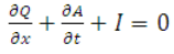      (31.1)

The momentum equation expressing the dynamic equilibrium of the flow process is:

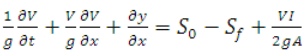     (31.2)

Where,   y - Depth of flow (m)

t -Time from beginning of irrigation (sec)

v - Velocity of flow as f (x, t) (m/s)

x - Distance along the furrow length (m)

I - Infiltrations rate as f (x, t) (m/s)

g - Acceleration due to gravity (m/s²)

S_o- Longitudinal slope of furrow (m/m)

S_f- Slope of energy grade line (friction slope) in (m/m)

A - Cross-sectional area as f (x, t) (m²)

Q - The discharge (m³/s)
These equations are first-order nonlinear partial differential Eq. without a known closed-form solution. Appropriate conversion or approximations of these equations are required. So, several mathematical simulation models (Full hydrodynamic, zero-inertia, kinematic-wave and volume-balance) have been developed, however, among them volume balance models are more commonly used for design. The volume balance models consider only the continuity eq. (31.1) and ignore the momentum eq. (31.2).

Empirical Infiltration Equation

Infiltration rate affects surface flow as well as performance of irrigation. Several expressions have been proposed for expressing infiltration rate as a function of elapsed time.

31.1.1 The Lewis- KostiakovEquation
A widely used empirical expression, for design of surface irrigation system, was originally proposed by Lewis (1937) but was erroneously attributed to Kostiakov.

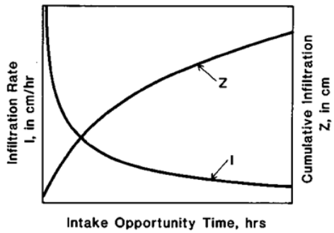
Fig.31.1.Infiltration rate and Cumulative infiltration vs. elapsed time. 

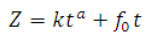
Cumulative:   Z = kt^a      (31.3)

      (31.4)

Where, Z= the cumulative depth of infiltration or the volume of water per unit soil surface area
t = elapsed time

k and a = empirical parameters

i = the infiltration rate

Disadvantages of the original Lewis- Kostiakov Equation

• It doesn't account for different initial soil water contents.
• For long infiltration times it erroneously predicts zero rate. 

Infiltration rate never becomes zero instead it reaches a steady state or constant rate condition after a long time. Therefore, the above Eq. was modified to reflect the steady state infiltration rate which may occur during surface irrigation system with longer set times.

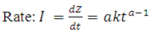
31.1.2 Modified KostiakovEquation

The later problem can be fixed by adding a parameter representing a final infiltration rate (constant infiltration rate) to the previous Eq. (31.1) and (31.2). So the equation becomes:

Z = kt^a + f_o t     (31.5)

     (31.6)

• Because of its simplicity, this model is frequently used in agricultural irrigation studies.
• Parameters k and a can be estimated by plotting the infiltration rate (I) or cumulative infiltration (Z) against time on log-log paper and fitting a straight line.

31.2 Volume Balance Concept

Volume balance equation

       (31.7)

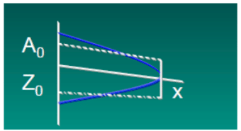
Fig. 31.2.Approximation of sub-surface and surface profiles during volume-balance. 

Also assume that advance characteristics follow a power function

 x = pt^r        (31.8)      

Power Advance Volume Balance Model
Using power advance, Elliott and Walker (1982) gave the following solution to the volume balance considering Modified Kostiakoveq:

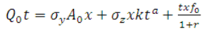          (31.9)

Where,  Q₀ = inflow rate, m³/min

A₀ = cross sectional area of flow inlet, m²

x = the advance distance, m

t= the advance time to distance x since beginning of irrigation, min

k and a= coefficients of modified Kostikov’s Eq.

f₀= basic infiltration rate, m³/m/min

p and r =empirical parameters of advance curve

σ_y =surface storage factor and generally it has a value of 0.77

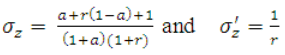
σzis defined as:

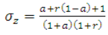    (31.10)

31.3 Advance Time Determination
Water will be distributed within a surface-irrigated field non-uniformly due to the differential time required for water to cover the field. To account for these differences in the design procedures, it is necessary to calculate the advance trajectory (curve).
It is first necessary to describe the flow cross section using two of the following functions:

A = a₁ y^a2     (31.11)

And

WP = b₁y^b2      (31.12)

Or as a simpler substitute,
AR^0.67 = p₁A^p2        (31.13)

Where,                
A= cross sectional flow area, m²
R = hydraulic radius, m
y = flow depth, m
WP= wetted perimeter, m
a₁, a₂, b₁, b₂, p₁,p₂ = empirical shape coefficients
For border and basin systems,a₁, a₂, b₁  and p₁ are equal to 1. The value of b₂ is 0.0 and p₂  is 3.3333.
The next step is to determine the cross-sectional flow area at the field inlet . For sloping fields, this can be accomplished with the Manning Eq. as follows:

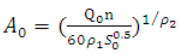         (31.14)

Where,                          
Q₀ = Field inlet discharge, m³/min/unit width
n = Manning roughness coefficient
S₀  = field slope
The design input data required at this point are , field length (L), S, nand . This information can be used to solve the volume balance Eq. for the time of advance,

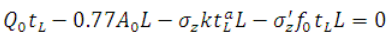    (31.15)

Where,      

Computation Steps of Advance Time

• The first step is to compute the flow cross-sectional area
• Make an initial estimate of power advance exponent (r) and label this value , usually setting ,  = 0.1 to 0.9 are good initial estimates. Then, a revised estimate of r is computed and compared below.
• Calculate the subsurface shape factors
• Calculate the time of advance by Newton- Raphson technique.
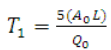
• Assume an initial estimate of t_L as T₁, Then
• Compute a revised estimate of t_L (say T₂) as,

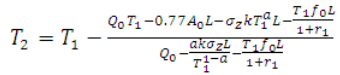    (31.16)

• Compare the initial and revised  of . If they are within about 0.5 minutes or less, the analysis proceeds to step 4. If they are not equal, let T₁ = T₂ and repeat steps b through c. It should be noted that if the inflow is insufficient to complete the advance phase in about 24 hours, the value of   is too small or the value of L is too large and the design process should be restarted with revised values. This can be used to evaluate the feasibility of a flow value and to find the inflow.
• Compute the time of advance to the field midpoint , using the same procedure as outlined in Step 4.

• The half-length (0.5L) is substituted for ‘L’ and ‘ ’ for ‘ ’.

• Volume balance Eq. is used with half length (0.5L) to find an appropriate value of

• Compute a revised estimate of ‘r’ say
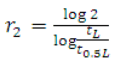            (31.17)
• Compare the initial estimate  with the revised estimate

• If the difference between the two values is less than 0.0001 (error criterion), the procedure for finding  is concluded.

• If not then  is replaced with  and steps 3-6 are repeated until the prescribed error criterion is satisfied.

31.4 Intake Opportunity Time Determination

The basic mathematical model of infiltration utilized in the intake opportunity time determination is the Kostiakov- Lewis relation:

 (31.18)

Where,    Z- required infiltrated volume per unit length, m³/m
(per furrow or per unit   width are implied)
t- The design intake opportunity time, minute
a -The constant exponent
k - The constant coefficient, m³/mina/m of length
f_o - the basic intake rate, m³/min/m of length
In order to express intake as a depth of application, Z must be divided by the unit width. For furrows, the unit width is the furrow spacing, w, while for borders and basins it is 1.0. Values of k, a, f_o and w along with the volume per unit length required to refill the root zone, Z_req, are design input data.
The volume balance design procedure requires that the intake opportunity time associated with  be known. This time, represented by can be obtained from modified Kostiakov Eq. using the Newton-Raphson procedure.