Earth Pressure Theories | Soil Mechanics - Civil Engineering (CE) PDF Download

Rankine's Earth Pressure Theory
Rankine's theory assumes that there is no wall friction (δ = 0), the ground and failure surfaces are straight planes, and that the resultant force acts parallel to the backfill slope.
In the case of retaining structures, the earth retained may be filled up the earth or natural soil. These backfill materials may exert certain lateral pressure on the wall. If the wall is rigid and does not move with the pressure exerted on the wall, the soil behind the wall will be in a state of elastic equilibrium. Consider the prismatic element E in the backfill at depth, z, as shown in Fig.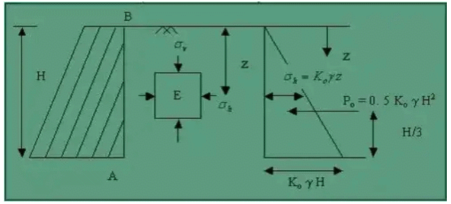
The element E is subjected to the following pressures:
Vertical pressure = σ = yz
Lateral pressure = σk, where g is the effective unit weight of the soil.
If we consider the backfill is homogenous, then both σv and σk increases rapidly with depth z. In that case, the ratio of vertical and lateral pressures remain constant with respect to depth, that is σk / σv = σk / yz = constant = Kϕ, where Kϕ is the coefficient of earth pressure for at-rest condition.
Earth Pressure at Rest
The at-rest earth pressure coefficient (Kϕ) is applicable for determining the active pressure in clays for strutted systems. Because of the cohesive property of clay, there will be no lateral pressure exerted in the at-rest condition up to some height when the excavation is made. However, with time, creep and swelling of the clay will occur, and lateral pressure will develop. This coefficient takes the characteristics of clay into account and will always give a positive lateral pressure.
The lateral earth pressure acting on the wall of height H may be expressed as σk = KϕyH.
The total pressure for the soil at rest condition, Pϕ = 0.5KϕyH2.
The value of Kϕ depends on the relative density of sand and the process by which the deposit was formed. If this process does not involve artificial tamping, the value of Kϕ ranges from 0.4 for loose sand to 0.6 for dense sand. Tamping of the layers may increase it upto 0.8.
From elastic theory, Kϕ = μ/(1 - μ), where μ is the Poisson's ratio.
According to Jaky (1994), a good approximation of Kϕ is given by, Kϕ = 1 - sinϕ.
- Rankine's Earth Pressure Against A Vertical Section With The Surface Horizontal With Cohesionless Backfill
(i) Active earth pressure: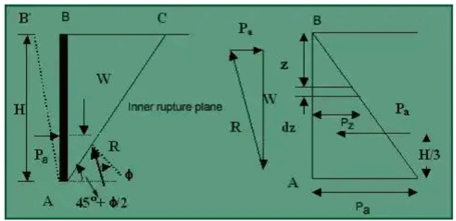 (a) Rankine's active earth pressure in the cohesionless soil
The lateral pressure acting against a smooth wall AB is due to the mass of soil ABC above the rupture line AC, which makes an angle of (45° + ϕ/2) with the horizontal. The lateral pressure distribution on the wall AB of height H increases in the same proportion to depth.
The pressure acts normal to the wall AB.
The lateral active earth pressure at A is Pa = KAyH, which acts at a height H/3 above the base of the wall.
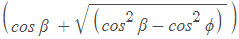
The total pressure on AB is therefore calculated as follows: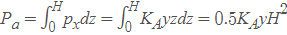 , where KA = tan2 (45° + ϕ/2)
(ii) Passive earth pressure: (a) Rankine's passive earth pressure in cohesionless soil
If the wall AB is pushed into the mass to such an extent as to impart a uniform compression throughout the mass, the soil wedge ABC in fig. will be in Rankine's Passive State of plastic equilibrium. The inner rupture plane AC makes an angle (45° + ϕ/2) with the vertical AB. The pressure distribution on the wall is linear, as shown.
The lateral passive earth pressure at A is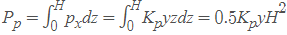 , where Kp = tan2 (45° + ϕ/2)
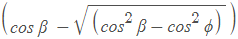
 - Rankine's active earth pressure with a sloping cohesionless backfill surface
As in the case of horizontal backfill, an active case of plastic equilibrium can be developed in the backfill by rotating the wall about A away from the backfill. Let AC be the plane of rupture, and the soil in the wedge ABC is in the state of plastic equilibrium.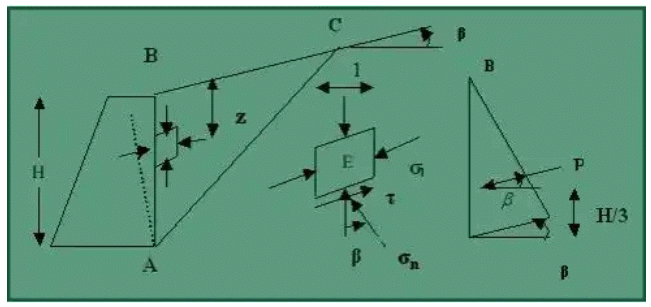 The pressure distribution on the wall is shown in fig. The active earth pressure at depth H is Pa = KAyH which acts parallel to the surface. The total pressure per unit length of the wall is Pa = 0.5KAyH2, which acts at the height of H/3 from the base of the wall and parallel to the sloping surface of the backfill.
In case of active pressure,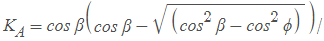
 .
.
In the case of Passive pressure,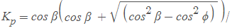
- Rankine's active earth pressures of cohesive soils with horizontal backfill on smooth vertical walls
In the case of cohesionless soils, the active earth pressure at any depth is given by Pa = KA yz. In the case of cohesive soils, the cohesion component is included, and the expression becomes Pa = KAYZ - 2c√KA.
When Pa = 0,z = zϕ = (2c√KA) / y.
This depth is known as the depth of the tensile crack. Assuming that the compressive force balances the tensile force (-), the total depth where tensile and compressive force neutralizes each other is 2zo. This is the depth up to which soil can stand without any support and is sometimes referred to as the depth of vertical crack or critical depth (Hc)(Hc = 4c√KA) / y.
However, Terzaghi, from field analysis, obtained that (Hc = 4c√KA) / y - zϕ, where zϕ ∼ Hc / 2 is not more than that.
The Rankine formula for passive pressure can only be used correctly when the embankment slope angle equals zero or is negative. If a large wall friction value can develop, the Rankine Theory will not correct and give less conservative results. Rankine's theory is not intended to determine earth pressures directly against a wall (friction angle does not appear in equations above). The theory is intended to determine earth pressures on a vertical plane within a mass of soil.
Coulomb's Wedge Theory
Coulomb (1776) developed a method for determining the earth pressure, in which he considered the equilibrium of the sliding wedge, which is formed when the movement of the retaining wall takes place. The sliding wadge is torn off from the rest of the backfill due to the movement of the wall. In the Active Earth pressure case, the siding wedge moves downwards & outwards on a slip surface relative to the intact backfill & in the case of Passive Earth pressure, the sliding wedge moves upward and inwards. The pressure on the wall is, in fact, a force of reaction which it has to exert to keep the sliding wedge in equilibrium. The lateral pressure on the wall is equal and opposite to the reactive force exerted by the wail in order to keep the siding wedge in equilibrium. The analysis is a type of limiting equilibrium method.
The following assumptions are made:
- The backfill is dry, cohesion lass, homogeneous, isotropic and ideally plastic material, elastically undeformable but breakable.
- The slip surface is a plane surface that passes through the hee! of the wall.
- The wall surface is rough. The resultant earth pressure on the wall is inclined at an angle δ to the normal to the wall, where δ is the angle of the friction between the wall and backfill.
- The sliding wedge itself acts as a rigid body & the value of the earth pressure is obtained by considering the limiting equilibrium of the sliding wedge as a whole.
- The position and direction of the resultant earth pressure are known. The resultant pressure acts on the back of the wall at one-third height of the wall from the base and is inclined at an angle δ to the normal to the back. This angle is called the angle of wall friction.
- The back of the wall is rough & the relative movement of the wall and the soil on the back takes place, which develops frictional forces that influence the direction of the resultant pressure.
Some Graphical solutions for lateral Earth Pressure are
- Culman's solution
- The trial wedge method
- The logarithmic spiral
|
30 videos|126 docs|74 tests
|
FAQs on Earth Pressure Theories - Soil Mechanics - Civil Engineering (CE)
| 1. What is earth pressure in civil engineering? |  |
| 2. What are the different types of earth pressure theories in civil engineering? | |
| 3. How does Rankine's theory of earth pressure differ from Coulomb's theory? | |
| 4. What is the Modified Coulomb's theory of earth pressure? | |
| 5. How is earth pressure calculated in civil engineering? | |


ppt
,past year papers
,Semester Notes
,Free
,Earth Pressure Theories | Soil Mechanics - Civil Engineering (CE)
,Exam
,Extra Questions
,Summary
,Sample Paper
,Earth Pressure Theories | Soil Mechanics - Civil Engineering (CE)
,shortcuts and tricks
,Viva Questions
,MCQs
,study material
,Important questions
,practice quizzes
,video lectures
,Previous Year Questions with Solutions
,mock tests for examination
,Objective type Questions
,Earth Pressure Theories | Soil Mechanics - Civil Engineering (CE)
;


Earth Pressure Theories Free PDF Download
Importance of Earth Pressure Theories
Earth Pressure Theories Notes
Earth Pressure Theories Civil Engineering (CE) Questions
Study Earth Pressure Theories on the App
|
© EduRev
|
Education Revolution
|


|


