Tacheometry, Plane Table & Curves | Geomatics Engineering (Surveying) - Civil Engineering (CE) PDF Download

Tacheometric Surveying
Tacheometry or telemetry is a branch of angular surveying in which the horizontal and vertical distances of points are obtained by optical means as opposed to the ordinary slower process of measurements by tape or chain.
- The method is very rapid and convenient.
- It is best adapted in obstacles such as steep and broken ground, deep ravines, stretches of water or swamp and so on, which make chaining difficult or impossible.
Tacheometry (from Greek, quick measure), is a system of rapid surveying, by which the positions, both horizontal and vertical, of points on the earth surface relatively to one another are determined without using a chain or tape or a separate leveling instrument.
Uses of Tacheometry
The tacheometric methods of surveying are used with an advantage over the direct methods of measurement of horizontal distances and differences in elevations.
Some of the uses are:
- Preparation of topographic maps which require both elevations and horizontal distances.
- Survey work in difficult terrain where direct methods are inconvenient
- Detail filling
- Reconnaissance surveys for highways, railways, etc.
- Checking of already measured distances
- Hydrographic surveys and
- Establishing secondary control.
Instrument
- An ordinary transit theodolite fitted with a stadia diaphragm is generally used for tacheometric survey.
- The stadia diaphragm essentially consists of one stadia hair above and the other an equal distance below the horizontal cross-hair, the stadia hairs being mounted in the ring and on the same vertical plane as the horizontal and vertical cross-hairs.
Different types of stadia hairs are shown below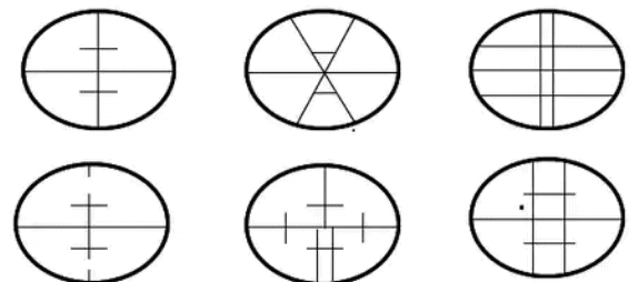
Methods of Tachometric Survey
Various methods of tacheometry survey are based on the principle that the horizontal distance between an instrument Station “A” and a staff station “B” depending on the angle subtended at point “A” by a known distance at point “B” and the vertical angle from point “B” to point “A” respectively.
This principle is used in different methods in different ways.
Mainly there are two methods of tachometry survey:
- Stadia system
- Tangential system
1. Stadia System of Tacheometry
In the stadia system, the horizontal distance to the staff Station from the instrument station and the elevation of the staff station concerning the line of sight of the instrument is obtained with only one observation from the instrument Station.
In the stadia method, there are mainly two systems of surveying.
- Fixed hair method
- Movable hair method (subtense method)
(i) Fixed Hair Method
- In the fixed hair method of tacheometric surveying, the instrument employed for taking observations consist of a telescope fitted with two additional horizontal cross hairs one above and the other below the central hair.
- These are placed equidistant from the central hair and are called stadia hairs.
- When a staff is viewed through the telescope, the stadia hairs are seen to intercept a certain length of the staff, and this varies directly with the distance between the instrument and the stations.
- As the distance between the stadia hair is fixed, this method is called the “fixed hair method.”
(a) Principle of Stadia Hair Method
- The stadia method is based on the principle that the ratio of the perpendicular to the base is constant in similar isosceles triangles.
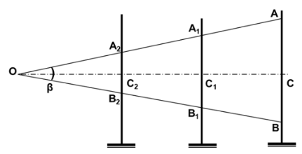
- In the figure, let two rays OA and OB be equally inclined to central ray OC.
- Let A2B2, A1B1, and AB be the staff intercepts. Evidently,
OC2/A2B2 = OC1/A1B1 = OC/AB = constant (k) = ½ cotβ/2
This constant k entirely depends upon the magnitude of the angle β
- In actual practice, observations may be made with either horizontal line of sight or with an inclined line of sight.
- In the latter case, the staff may be kept either vertically or normal to the line of sight.
- First, the distance-elevation formulae for the horizontal sights should be derived.
(b) Horizontal Line of Sight
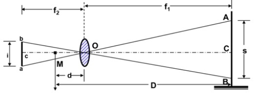
Consider the figure, in which O is the optical center of the objective of an external focusing telescope.
- Let A, C, and B be the points cut by the three lines of sights corresponding to three wires.
- b, c, and a be top, axial and bottom hairs of the diaphragm.
ab = i = interval b/w the stadia hairs (stadia interval)
AB = s = staff intercept,
f = focal length of the objective
f1 = horizontal distance of the staff from the optical center of the objective
f2 = horizontal distance of the cross-wires from O.
d = distance of the vertical axis of the instrument from O.
D = horizontal distance of the staff from the vertical axis of the instruments.
M = center of the instrument, corresponding to the vertical axis.
Horizontal distance between the axis and the staff is
D = (f/i)s + (f + d) = k.s + C
Above equation is known as the distance equation. In order to get the horizontal distance, therefore, the staff intercept s is to be found by subtracting the staff readings corresponding to the top and bottom stadia hairs.
- The constant k = f/i is known as the multiplying constant or stadia interval factor and the constant (f + d) = C is known as the additive constant of the instrument.
(c) Inclined Line of Sight (staff held vertical)
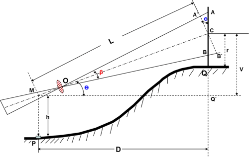
MC = L = k.S.Cosθ + C
Horizontal Distance
MQ’ = D = L.Cosθ
Vertical Distance
CQ’ = V = L.Sinθ
Elevation of the staff station for the angle of elevation:
If the line of sight has an angle of elevation θ, as shown in the figure, we have
Elevation of staff station = Elevation of instrument station + h + V – r.
Elevation of the staff station for the angle of depression:
Elevation of Q = Elevation of P + h – V - r
(d) Inclined Line of Sight (staff held normal to the sight)
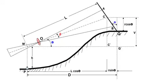
Case(a): Line of Sight at an angle of elevation Θ
Let AB = s = staff intercept;
CQ = r = axial hair reading
With the same notations as in the last case, we have
MC = L = Ks + C
The horizontal distance between P and Q is given by
D = MC' + C'Q' = LcosΘ + rsinΘ
=(k s + C)cosΘ + rsinΘ
Similarly, V = lsinΘ = (k s + C) sinΘ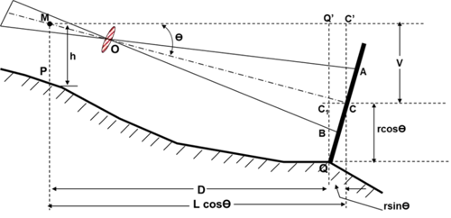
Case(b): Line of Sight at an angle of depressionθ
Figure shows the line of sight depressed downwards,
MC = L = k s + C
D = MQ' = MC' - Q'C'
= L cosΘ - r sinΘ
D = (k s + C)cosΘ - r sin Θ
V = L sin Θ = (k s + C) sin Θ
Elevation of Q = Elevation of P + h - V - r cosΘ
(ii) Movable Hair Method (Subtense Method)
In the movable Hair method of tacheometric surveying, the instrument used for taking observations consist of a telescope fitted with stadia hairs which can be moved and fixed at any distance from the central hair (within the limits of the diaphragm).
The staff used with this instrument consists of two targets (marks) at a fixed distance apart (say 3.4 mm).
The Stadia interval which is variable for the different positions of the staff is measured, and the horizontal distance from the instrument station to the staff station is computed.
Note: Out of the two methods mentioned above of tacheometric surveying, the “fixed hair method “is widely employed.
2. Tangential System of Tacheometric Surveying
- In this system of tacheometric surveying, two observations will be necessary from the instrument station to the staff station to determine the horizontal distance and the difference in the elevation between the line of collimation and the staff station.
- The only advantage of this method is that this survey can be conducted with ordinary transit theodolite.
- As the ordinary transit theodolite is cheaper than the intricate and more refined tacheometer, so, the survey will be more economical.
- So, as far as the reduction of field notes, distances and elevations are concerned there is not much difference between these two systems.
- But this system is considered inferior to the stadia system due to the following reasons and is very seldom used nowadays.
- This involves the measurement of two vertical angles, and the instrument may get disturbed between the two observations.
- The speed is reduced due to a greater number of observations and the changes in the atmospheric conditions will affect the readings considerably.
- The staff used in this method is similar to the one employed in the movable hair method of stadia surveying. The distance between the targets or vanes may be 3-4 m.
Case 1: When both angles are above the horizontal line of sight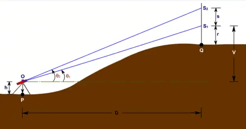
V = D tanθ1
V + s = D tanθ2
Thus, s = D ( tanθ2 - tanθ1)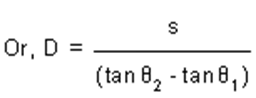
- Therefore R.L. of Q = (R.L. of P + h) + V – r
- where h is the height of the instrument, r is the staff reading corresponding to the lower vane.
Case 2: When both angles are below the horizontal line of sight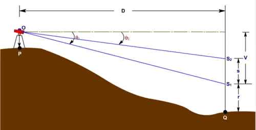
- V = D tanθ1
- V-s = D tanθ2
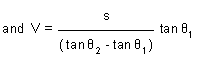
Thus, s = D ( tanθ1 - tanθ2)
Or D = s/(tanθ2 - tanθ1)
and V = (s/tanθ1 - tanθ2))tanθ1
Therefore R.L. of Q = (R.L. of P + h) - V – r
where h is the height of the instrument, r is the staff reading corresponding to the lower vane.
Case 3: When one angle is above and one angle is below the horizontal line of sight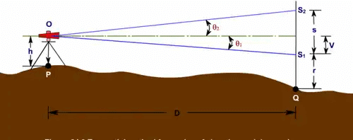
- V = D tan q1
- s - V = D tanθ2
Thus, s = D (tanθ2 + tanθ1)
Or, D = S/(tanθ2 + tanθ1)
and, V = (s/(tanθ2 + tanθ1))tanθ1
Therefore R.L. of Q = (R.L. of P + h) - V – r
where h is the height of the instrument, r is the staff reading corresponding to the lower vane.
|
19 videos|59 docs|35 tests
|
FAQs on Tacheometry, Plane Table & Curves - Geomatics Engineering (Surveying) - Civil Engineering (CE)
| 1. What is tacheometric surveying? |  |
| 2. What is the role of a plane table in tacheometric surveying? | |
| 3. How does tacheometry help in the construction of curves in civil engineering? | |
| 4. What are the advantages of tacheometric surveying over traditional methods? | |
| 5. How can tacheometry be applied in the field of civil engineering? | |


mock tests for examination
,Tacheometry
,video lectures
,Tacheometry
,MCQs
,Semester Notes
,Viva Questions
,Objective type Questions
,Sample Paper
,Exam
,past year papers
,ppt
,Tacheometry
,Summary
,shortcuts and tricks
,Previous Year Questions with Solutions
,Extra Questions
,Plane Table & Curves | Geomatics Engineering (Surveying) - Civil Engineering (CE)
,Plane Table & Curves | Geomatics Engineering (Surveying) - Civil Engineering (CE)
,Free
,Important questions
,Plane Table & Curves | Geomatics Engineering (Surveying) - Civil Engineering (CE)
,study material
,practice quizzes
;


Tacheometry, Plane Table & Curves Free PDF Download
Importance of Tacheometry, Plane Table & Curves
Tacheometry, Plane Table & Curves Notes
Tacheometry, Plane Table & Curves Civil Engineering (CE) Questions
Study Tacheometry, Plane Table & Curves on the App
|
© EduRev
|
Education Revolution
|


|


