Civil Engineering (CE) Exam > Civil Engineering (CE) Notes > Environmental Engineering > Water Demand
Water Demand | Environmental Engineering - Civil Engineering (CE) PDF Download

Fire Demand
Rate of fire demand is sometimes treated as a function of population and is worked out on the basis of empirical formulas:
- As per GO Fire Demand
= 100(P)1/2 - Kuichling’s Formula
Where Q = Amount of water required in liters/minute.
P = Population in thousand. - Freeman Formula

- National Board of Fire Under Writers Formula
(i) For a central congested high valued city
(a) Where population < 200000
(b) where population > 200000
Q = 54600 lit/minute for first fire
and Q = 9100 to 36,400 lit/minute for a second fire.
(ii) For a residential city.
(a) Small or low building,
Q = 2,200 lit/minutes.
(b) Larger or higher buildings,
Q = 4500 lit/minute.
(c) High value residences, apartments, tenements
Q = 7650 to 13,500 lit/minute.
(d) Three storeyed buildings in density built-up sections,
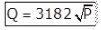
Q = 27000 lit/minute. - Buston’s Formula

The probability of occurrence of a fire, which, in turn, depends upon the type of the city served, has been taken into consideration in developing a above formula on the basis of actual water consumption in fire fighting for Jabalpur city of India. The formula is given as
Where,
R = Recurrence interval of fire i.e., period of occurrence of fire in years, which will be different for residential, commercial and industrial cities.
Per Capita Demand (q)

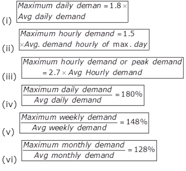
Assessment of Normal Variation
Population forecasting Methods
- Arithmetic increase method

Where,
Prospective or forecasted population after n decades from the present (i.e., last known census)
Population at present (i.e., last known census)
n = Number of decades between now & future.
Average (arithmetic mean) of population increases in the known decades. - Geometric Increase Method

where,
Po = Initial population.
Pn = Future population after ‘n’ decades.
r = Assumed growth rate (%).
where,
P2 = Final known population
P1 = Initial known population
t = Number of decades (period) between P1 and P2.
- Incremental Increases Method

Where, Average increase of population of known decades
 Average of incremental increases of the known decades.
 - Decreasing rate of growth method
Since the rate of increase in the population goes on reducing, as the cities reach towards saturation, a method which makes use of the decrease in the percentage increase, in many times used, and gives quite rational results. In this method, the average decrease in the percentage increase is worked out, and is then subtracted from the latest percentage increase for each successive decade. This method is, however, applicable only in cases, where the rate of growth shows a downward trend. - Logistic Curve Method
(a)
Where,
Po = Population of the start point.
Ps = Saturation population
P = Population at any time t from the origin.
k = Constant.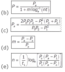
The document Water Demand | Environmental Engineering - Civil Engineering (CE) is a part of the Civil Engineering (CE) Course Environmental Engineering.
All you need of Civil Engineering (CE) at this link: Civil Engineering (CE)
|
14 videos|120 docs|98 tests
|
FAQs on Water Demand - Environmental Engineering - Civil Engineering (CE)
| 1. What is water demand in civil engineering? |  |
Ans. Water demand in civil engineering refers to the quantity of water required for various activities such as domestic use, industrial processes, irrigation, and firefighting. It is an essential factor in designing water supply systems and ensuring the availability of sufficient water resources to meet the needs of a specific area or project.
| 2. How is water demand calculated in civil engineering projects? | |
Ans. Water demand in civil engineering projects is calculated by considering various factors such as population growth, per capita water consumption, and specific water requirements for different activities. The calculation involves estimating the water demand for each category and then summing them up to determine the total water demand for the project.
| 3. What are the factors influencing water demand in civil engineering? | |
Ans. Several factors influence water demand in civil engineering, including population growth, urbanization, climate conditions, economic development, lifestyle patterns, and technological advancements. These factors affect the overall water consumption and usage patterns, thereby impacting the estimation of water demand for a particular project or area.
| 4. How is water demand forecasted in civil engineering? | |
Ans. Water demand forecasting in civil engineering involves analyzing historical water consumption data, considering the population growth rate, and evaluating the impact of various factors like climate change and socio-economic conditions. Statistical models and simulation techniques are commonly used to forecast future water demand, helping in the planning and design of water supply systems.
| 5. What are some strategies to manage water demand in civil engineering projects? | |
Ans. To manage water demand in civil engineering projects, several strategies can be adopted, including:
- Implementing water-efficient fixtures and appliances in buildings to reduce water consumption.
- Promoting water conservation practices such as rainwater harvesting and greywater recycling.
- Educating the community about the importance of water conservation and encouraging responsible water use.
- Enhancing water infrastructure and distribution systems to minimize water losses and leakage.
- Implementing water pricing mechanisms and incentives to encourage efficient water use.
About this Document

1.1K Views

4.65/5
Rating

Oct 18, 2025
Last updated
Related Exams
Document Description: Water Demand for Civil Engineering (CE) 2025 is part of Environmental Engineering preparation.
The notes and questions for Water Demand have been prepared according to the Civil Engineering (CE) exam syllabus. Information about Water Demand covers topics
like and Water Demand Example, for Civil Engineering (CE) 2025 Exam. Find important definitions, questions, notes, meanings, examples, exercises and tests below for Water Demand.
Introduction of Water Demand in English is available as part of our Environmental Engineering
for Civil Engineering (CE) & Water Demand in Hindi for Environmental Engineering course.
Download more important topics related with notes, lectures and mock test series for Civil Engineering (CE)
Exam by signing up for free. Civil Engineering (CE): Water Demand | Environmental Engineering - Civil Engineering (CE)
Description
Full syllabus notes, lecture & questions for Water Demand | Environmental Engineering - Civil Engineering (CE) - Civil Engineering (CE) | Plus excerises question with solution to help you revise complete syllabus for Environmental Engineering | Best notes, free PDF download
Information about Water Demand
In this doc you can find the meaning of Water Demand defined & explained in the simplest way possible. Besides explaining types of
Water Demand theory, EduRev gives you an ample number of questions to practice Water Demand tests, examples and also practice Civil Engineering (CE)
tests

Related Searches
MCQs
,Water Demand | Environmental Engineering - Civil Engineering (CE)
,Sample Paper
,mock tests for examination
,past year papers
,video lectures
,Water Demand | Environmental Engineering - Civil Engineering (CE)
,study material
,Extra Questions
,Viva Questions
,Previous Year Questions with Solutions
,Objective type Questions
,practice quizzes
,Important questions
,shortcuts and tricks
,Free
,Semester Notes
,Water Demand | Environmental Engineering - Civil Engineering (CE)
,ppt
,Exam
,Summary
;


Additional Information about Water Demand for Civil Engineering (CE) Preparation
Water Demand Free PDF Download
The Water Demand is an invaluable resource that delves deep into the core of the Civil Engineering (CE) exam.
These study notes are curated by experts and cover all the essential topics and concepts, making your preparation more efficient and effective.
With the help of these notes, you can grasp complex subjects quickly, revise important points easily,
and reinforce your understanding of key concepts. The study notes are presented in a concise and easy-to-understand manner,
allowing you to optimize your learning process. Whether you're looking for best-recommended books, sample papers, study material,
or toppers' notes, this PDF has got you covered. Download the Water Demand now and kickstart your journey towards success in the Civil Engineering (CE) exam.
Importance of Water Demand
The importance of Water Demand cannot be overstated, especially for Civil Engineering (CE) aspirants.
This document holds the key to success in the Civil Engineering (CE) exam.
It offers a detailed understanding of the concept, providing invaluable insights into the topic.
By knowing the concepts well in advance, students can plan their preparation effectively.
Utilize this indispensable guide for a well-rounded preparation and achieve your desired results.
Water Demand Notes
Water Demand Notes offer in-depth insights into the specific topic to help you master it with ease.
This comprehensive document covers all aspects related to Water Demand.
It includes detailed information about the exam syllabus, recommended books, and study materials for a well-rounded preparation.
Practice papers and question papers enable you to assess your progress effectively.
Additionally, the paper analysis provides valuable tips for tackling the exam strategically.
Access to Toppers' notes gives you an edge in understanding complex concepts.
Whether you're a beginner or aiming for advanced proficiency, Water Demand Notes on EduRev are your ultimate resource for success.
Water Demand Civil Engineering (CE) Questions
The "Water Demand Civil Engineering (CE) Questions" guide is a valuable resource for all aspiring students preparing for the
Civil Engineering (CE) exam. It focuses on providing a wide range of practice questions to help students gauge
their understanding of the exam topics. These questions cover the entire syllabus, ensuring comprehensive preparation.
The guide includes previous years' question papers for students to familiarize themselves with the exam's format and difficulty level.
Additionally, it offers subject-specific question banks, allowing students to focus on weak areas and improve their performance.
Study Water Demand on the App
Students of Civil Engineering (CE) can study Water Demand alongwith tests & analysis from the EduRev app,
which will help them while preparing for their exam. Apart from the Water Demand,
students can also utilize the EduRev App for other study materials such as previous year question papers, syllabus, important questions, etc.
The EduRev App will make your learning easier as you can access it from anywhere you want.
The content of Water Demand is prepared as per the latest Civil Engineering (CE) syllabus.
|
© EduRev
|
Education Revolution
|


|


Signup on EduRev and stay on top of your study goals
10M+ students crushing their study goals daily