Compressibility & Consolidation of Soils | Soil Mechanics - Civil Engineering (CE) PDF Download

Compressibility and Consolidation 5
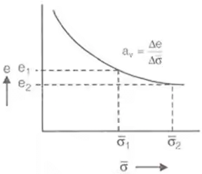
- Coefficient of Compressibility (av)
av = e1 - e2/σ2 - σ1
e1 = Void ratio at effective stress
e2 =Void ratio at effective stress
 ΔV/V0 = ΔH/H0
ΔV = Change in volume in m3, or cm3
V0 = Initial volume in m3 or cm3.
ΔH = Change in depth in 'm' or 'cm'.
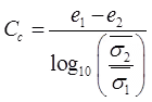
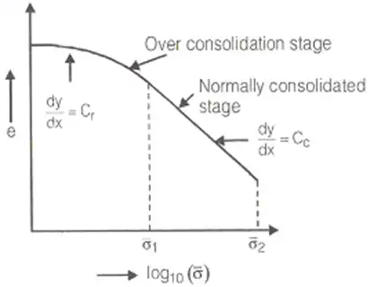
H0 = original depth in 'm' or 'cm'. - Coefficient of Compression (Cc)
(i)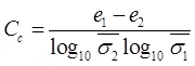
↓
(ii) Cc = 0.009(WL-10)
For undisturbed soil of medium sensitivity.
WL = % liquid limit.
(iii) Cc = 0.009(WL-7)
For remolded soil of low sensitivity
(iv) Cc = 0.40(e0-0.25)
For undisturbed soil of medium sensitivity e0 = Initial void ratio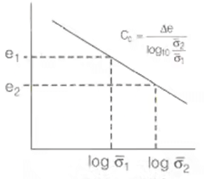 (v) For remoulded soil of low sensitivity.
Cc = 1.15(e0 - 0.35)
(vi) Cc = 0.115w where, w = Water content - Over consolidation ratio
O.C.R = Maximum effective stress applied in the past/Existing effective stress
O.C.R > 1 For over consolidated soil.
O.C.R = 1 For normally consolidated soil.
O.C.R < 1 For under consolidated soil.
Differential Equation of 1-D Consolidation
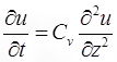 where, u = Excess pore pressure.
∂u / ∂t = Rate of change of pore pressure
Cv = Coefficient of consolidation
∂u / ∂z = Rate of change of pore pressure with depth.
- Coefficient of volume compressibility mv = av/1+e0 where, e0 = Initial void ratio
mv = Coefficient of volume compressibility
Compression modulus
Ec = 1/mv where, Ec =Compression modulus. - Degree of consolidation
(i) %U = (1-(U/U1)x100) where,
%U = % degree of consolidation.
U = Excess pore pressure at any stage.
U1 = = Initial excess pore pressure
at t = 0, u = u1 ⇒ %u = 0%
at t = ∞, u = 0 ⇒ %u = 100%
(ii) %u = (e0-e/e0-ef)x100 where,
ef = Void ratio at 100% consolidation.
i.e. of t = ∞
e = Void ratio at time 't'
e0 = Initial void ratio i.e., at t = 0
(iii) %u = (Δh / ΔH) x 100 where,
ΔH = Final total settlement at the end of completion of primary consolidation i.e.,
at t = ∞
Δh = Settlement occurred at any time 't'. - Time factor
Tv = Cv.(t/d2) where, TV = Time factor
CV = Coeff. of consolidation in cm2/sec.
d = Length of drainage path
t = Time in 'sec'
d = H0/2 For 2-way drainage
d = H0 For one-way drainage.
where, H0 = Depth of soil sample.
(i) Tv = (π/4)(u)2 ... if u ≤ 60% T50 = 0.196
(ii) Tv = -0.9332log10(1-u)-0.0851...
if u > 60%
Method to find 'Cv'
- Square Root of Time Fitting Method
Cv = (T90.d2)/t90 where,
T90 = Time factor at 90% consolidation
t90 = Time at 90% consolidation
d = Length of drainage path. - Logarithm of Time Fitting Method
Cv = T50.d2/t50
where, T50 = Time factor at 50% consolidation
t50 = Time of 50% consolidation.
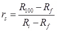
Compression Ratio
- Initial Compression Ratio
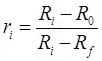
where, Ri = Initial reading of dial gauge.
R0 = Reading of dial gauge at 0% consolidation.
Rf = Final reading of dial gauge after secondary consolidation. - Primary Consolidation Ratio
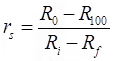
where, R100 = Reading of dial gauge at 100% primary consolidation. - Secondary Consolidation Ratio
 ri+rp+rs = 1
Total Settlement
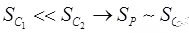
S = Si + Sp + Ss where, Si = Initial settlement
Sp = Primary settlement
Ss = Secondary settlement
- Initial Settlement
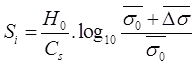
For cohesionless soil.
where, Cs = 1.5(Cr/σ0)
where, Cr = Static one resistance in kN/m2
H0 = Depth of soil sample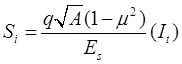 For cohesive soil.
where, It = Shape factor or influence factor
A = Area. - Primary Settlement
(i)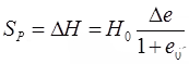
(ii)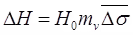
(iii)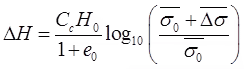
(iv)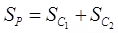
 = Settlement for over consolidated stage
 = Settlement for normally consolidation stage
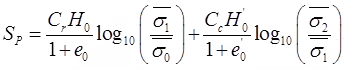
- Secondary Settlement
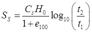
where, H0∼H100
H100 = Thickness of soil after 100% primary consolidation.
e100 = Void ratio after 100% primary consolidation.
t2 = Average time after t1 in which secondary consolidation is calculated
Permeability
- Permeability of Soil
The permeability of a soil is a property which describes quantitatively, the ease with which water flows through that soil. - Darcy's Law
Darcy established that the flow occurring per unit time is directly proportional to the head causing flow and the area of cross-section of the soil sample but is inversely proportional to the length of the sample.
(i) Rate of flow (q)
qα(Δh/L)A → q = KiA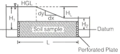 Where, q = rate of flow in m3/sec.
K = Coefficient of permeability in m/s
I = Hydraulic gradient
A = Area of cross-section of sample
i = HL/L where, HL = Head loss = (H1 – H2)
i = tanθ(dy/dx)
(ii) Seepage velocity
Vs = V/n where, Vs = Seepage velocity (m/sec)
n = Porosity & V = discharge velocity (m/s)
(iii) Coefficiency of percolation
KP = K/n where, KP = coefficiency of percolation and n = Porosity. - Constant Head Permeability Test
K = QL/tHLA where, Q = Volume of water collected in time t in m3.
Constant Head Permeability test is useful for coarse grain soil and it is a laboratory method.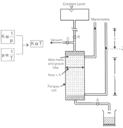
- Falling Head Permeability Test or Variable Head Permeability Test
K = 2.303aL/At(log10)(h1 / h2)
a = Area of tube in m2
A = Area of sample in m2
t = time in 'sec'
L = length in 'm'
h1 = level of upstream edge at t = 0
h2 = level of upstream edge after 't'.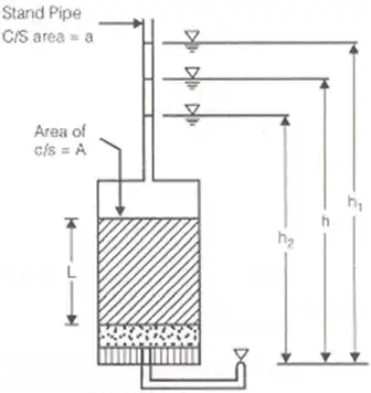
- Konzey-Karman Equation
Where, C = Shape coefficient, ∼5mm for spherical particle
S = Specific surface area = Area/Volume - For spherical particle.
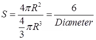
R = Radius of spherical particle.
S = 6/√ab
When particles are not spherical and of variable size. If these particles passes through sieve of size 'a' and retain on sieve of size 'n'.
e = void ratio
μ = dynamic viscosity, in (N - s/m2)
γw = unit weight of water in kN/m3
- Allen Hazen Equation
K=C.D210 Where, D10 = Effective size in cm. k is in cm/s C = 100 to 150 - Lioudens Equation
log10KS2= a + b.n
Where, S = Specific surface area
n = Porosity.
a and b are constant.
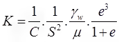
Consolidation equation K = Cvmvγw
Where, Cv = Coefficient of consolidation in cm2/sec
mv = Coefficient of volume Compressibility in cm2/N - Capillary Permeability Test
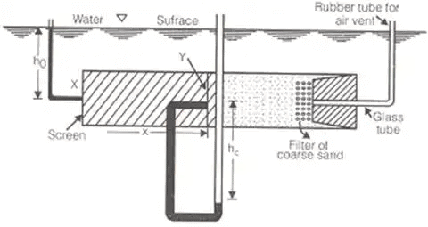 i = h0 + hc/x where, S = Degree of saturation
K = Coefficient of permeability of partially saturated soil.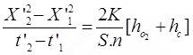
where hc = remains constant (but not known as depends upon soil)
= head under first set of observation,
n = porosity, hc = capillary height
Another set of data gives, = head under second set of observation
For S = 100%, K = maximum. Also, ku ∝ S. - Permeability of a stratified soil
(i) Average permeability of the soil in which flow is parallel to bedding plane,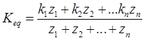 keq∼kx
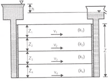 (ii) Average permeability of soil in which flow is perpendicular to bedding plane.
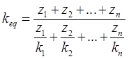 keq∼kz
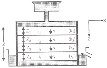 (iii) For 2-D flow in x and z direction
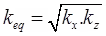
(iv) For 3-D flow in x, y and z direction keq = (kx.ky.kz)1/3
Coefficient of absolute permeability (k0)
Effective Stress, Capilarity, Seepage
- Seepage Pressure and Seepage Force
Seepage pressure is exerted by the water on the soil due to friction drag. This drag force/seepage force always acts in the direction of flow.
The seepage pressure is given by
PS = hγω where, Ps = Seepage pressure
γω = 9.81 kN/m3
Here, h = head loss and z = length
(i) FS = hAγω where, Fs = Seepage force
(ii) fs = iγω where, fs = Seepage force per unit volume.
i = h/z where, I = Hydraulic gradient. - Quick Sand Condition
It is condition but not the type of sand in which the net effective vertical stress becomes zero, when seepage occurs vertically up through the sands/cohesionless soils.
Net effective vertical stress = 0
ic = (G - 1)/(1 + e) where, ic = Critical hydraulic gradient.
2.65 ≤ G ≤ 2.70 0.65 ≤ e ≤ 0.70
To Avoid Floating Condition
i < i and F.O.S = ic/i > 1
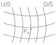
Laplace Equation of Two Dimensional Flow and Flow Net: Graphical Solution of Laplace Equation
(i) 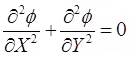
where, ∅ = Potential function = kH
H = Total head and k = Coefficient of permeability
(ii) 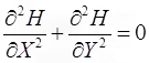 … 2D Laplace equation for Homogeneous soil.
where, ∅ = kX H and ∅ = ky H for Isotropic soil, kx= ky
Seepage discharge (q)
q = kh.(Nf/Nd) where, h = hydraulic head or head difference between upstream and downstream level or head loss through the soil.
- Shape factor = Nf/Nd
- Nf = Nψ - 1
where, Nf = Total number of flow channels
Nψ = Total number of flow lines. - Nd = N∅ - 1
where, Nd = Total number equipotential drops.
N∅ = Total number equipotential lines. - Hydrostatic pressure = U = hwγw
where, U = Pore pressure hw = Pressure head
hw = Hydrostatic head – Potential head - Seepage Pressure
Ps = h'γw where, h' = h - (2h/Nd)
- Exit gradient,
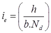 where, size of exit flow field is b x b.
and ΔH = h/Nd is equipotential drop.
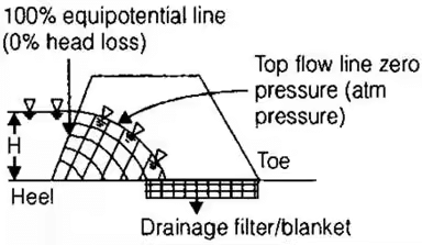
Phreatic Line
It is top flow line which follows the path of base parabola. It is a stream line. The pressure on this line is atmospheric (zero) and below this line pressure is hydrostatic.
- Phreatic Line with Filter
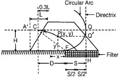 Phreatic line (Top flow line).
↓
Follows the path of base parabola
CF = Radius of circular arc =
C = Entry point of base parabola
F = Junction of permeable and impermeable surface
S = Distance between focus and directrix
= Focal length.
FH = S
(i) q = ks where, q = Discharge through unit length of dam.
(ii)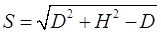
(iii)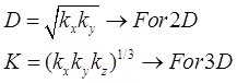
- Phreatic Line without Filter
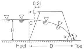 (i) For ∝ < 30°
q = k a sin2 ∝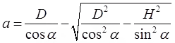
(ii) For ∝ > 30°
q = k a sin ∝ tan ∝ and
|
30 videos|126 docs|74 tests
|
FAQs on Compressibility & Consolidation of Soils - Soil Mechanics - Civil Engineering (CE)
| 1. What is compressibility of soils? |  |
| 2. How is compressibility of soils determined? | |
| 3. What is consolidation of soils? | |
| 4. How does consolidation affect the behavior of soils? | |
| 5. What factors influence the compressibility and consolidation of soils? | |


Exam
,Semester Notes
,Compressibility & Consolidation of Soils | Soil Mechanics - Civil Engineering (CE)
,Objective type Questions
,MCQs
,study material
,Free
,Viva Questions
,mock tests for examination
,Important questions
,Compressibility & Consolidation of Soils | Soil Mechanics - Civil Engineering (CE)
,Sample Paper
,Previous Year Questions with Solutions
,shortcuts and tricks
,Summary
,Extra Questions
,past year papers
,video lectures
,practice quizzes
,ppt
,Compressibility & Consolidation of Soils | Soil Mechanics - Civil Engineering (CE)
;


Compressibility & Consolidation of Soils Free PDF Download
Importance of Compressibility & Consolidation of Soils
Compressibility & Consolidation of Soils Notes
Compressibility & Consolidation of Soils Civil Engineering (CE) Questions
Study Compressibility & Consolidation of Soils on the App
|
© EduRev
|
Education Revolution
|


|


