Round Robin Scheduling

Program for Round Robin scheduling
Round Robin is a preemptive CPU scheduling algorithm in which each ready process is assigned a fixed time slice, called the time quantum, in a cyclic order. When a process's time quantum expires and it has not finished execution, it is preempted and placed at the end of the ready queue. This gives each process a fair share of the CPU and prevents starvation.
- Simple and easy to implement.
- Preemptive-a process runs only for at most one time quantum at a time.
- Starvation-free because of its cyclic (round-robin) nature; every process eventually receives CPU time.
- Commonly used in time-sharing systems and as the core technique in many general-purpose schedulers.
- Overhead: frequent context switches if the quantum is small, which reduces CPU efficiency.
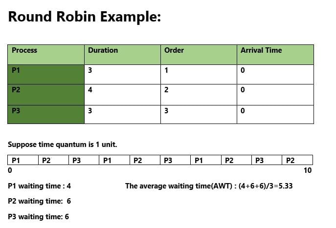
Illustration
Performance metrics and important times
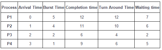
- Completion Time: the time at which a process finishes execution.
- Turnaround Time (TAT): total time a process spends in the system. TAT = Completion Time - Arrival Time
- Waiting Time (WT): total time a process spends waiting in the ready queue. WT = Turnaround Time - Burst Time
Note: If all processes have arrival time = 0, then Turnaround Time equals Completion Time for each process.
Computing waiting times (basic method when arrival times are 0)
To compute waiting times in Round Robin, maintain the remaining burst times and simulate the scheduler until all processes complete. The commonly used arrays and variables are:
- bt[] - original burst times of processes.
- rem_bt[] - remaining burst times; initially rem_bt[i] = bt[i].
- wt[] - waiting times; initialise wt[i] = 0 for all i.
- t - current time; initialise t = 0.
- quantum - time slice assigned to each process each turn.
Algorithm (simulation loop):
- Repeat while at least one rem_bt[i] > 0 for processes in the ready set:
- For each process i (in fixed cyclic order):
- If rem_bt[i] > 0 then:
- If rem_bt[i] > quantum, then
- t = t + quantum
- rem_bt[i] = rem_bt[i] - quantum
- Else (last cycle for that process):
- t = t + rem_bt[i]
- wt[i] = t - bt[i]
- rem_bt[i] = 0
- End for
- End repeat
After computing waiting times, compute turnaround times as tat[i] = wt[i] + bt[i]. Average waiting time and average turnaround time are obtained by summing these values over all processes and dividing by the number of processes.
Round Robin scheduling with different arrival times
When processes have different arrival times, the scheduler must also manage a dynamic ready queue. Key ideas and rules are:
- Add a process to the ready queue when its arrival time ≤ current time.
- When a process is running, if other processes arrive during its time quantum, those arriving processes are enqueued at the end of the ready queue.
- When the time quantum of the running process expires and it is not finished, move that process to the end of the ready queue.
- If the ready queue is empty and no process has arrived yet, the CPU remains idle until the next arrival; if the ready queue is empty but the current process still has remaining burst and its quantum has not expired, the process may continue (implementation detail) - typical implementations continue the current process only up to its quantum; if no other process is ready the next scheduling decision depends on the scheduler design.
- The scheduler continues until every process has completed.
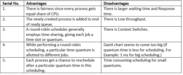
Properties, advantages and disadvantages
- Properties: cyclic, preemptive, fair to all processes, no priority by default (every process has equal importance in pure RR).
- Advantages: fair sharing of CPU; prevents starvation; simple to implement.
- Disadvantages: throughput and average waiting time depend strongly on quantum size; frequent context switches when the quantum is small; cannot provide different priorities to processes without modifications.
Effect of quantum selection: If the quantum is very large (larger than most burst times), RR approximates First-Come First-Served (FCFS). If the quantum is very small, RR behaves like processor sharing with high context-switch overhead, increasing effective execution time due to context switch cost. Choose quantum such that context-switch overhead remains small compared to useful work per quantum.
Example note: If quantum time = 2, each ready process can run for up to 2 time units per turn. New arrivals during those 2 units are appended to the ready queue and will get CPU in subsequent turns.
Step-by-step implementation approach (typical program structure)
- Declare arrays: arrival[], burst[], wait[], turn[], and initialise them. Create a copy rem_bt[] (or temp_burst[]) from burst[] to preserve original burst times for final calculations.
- Create a boolean array completed[] or a counter to track finished processes. Initialise a queue (or a circular array / linked list) to hold indices of ready processes.
- Initialise timer variable t = 0 and add any processes that have arrival time ≤ t to the ready queue.
- While there are unfinished processes do:
- If ready queue is empty, advance t to the next arrival time and enqueue newly arrived processes.
- Dequeue the first process index from ready queue and execute it for up to quantum time units. During execution, enqueue any processes that arrive.
- If the process finishes within the quantum, record its completion time and mark it complete. If it does not finish, reduce its remaining burst time and enqueue it at the end of the ready queue.
- Repeat until all processes are complete; then compute waiting times and turnaround times using recorded completion times and original burst/arrival times.
Pseudocode (concise)
Initialise rem_bt[i] = burst[i] for all i Initialise t = 0 Initialise ready queue Q Enqueue all processes with arrival[i] ≤ t into Q while (there exists i with rem_bt[i] > 0) { if Q is empty { advance t to next smallest arrival time not yet processed enqueue processes that have arrival time ≤ t continue } i = dequeue(Q) if rem_bt[i] > quantum { t = t + quantum rem_bt[i] = rem_bt[i] - quantum enqueue any newly arrived processes (arrival ≤ t) enqueue(i) // process goes to end of queue } else { t = t + rem_bt[i] rem_bt[i] = 0 completion[i] = t enqueue any newly arrived processes (arrival ≤ t) } } for each process i { tat[i] = completion[i] - arrival[i] wt[i] = tat[i] - burst[i] }
Practical tips for interview and examination
- Explain the role of the time quantum clearly and mention its effects on average waiting time, turnaround time and context switching overhead.
- Be prepared to simulate RR on a small set of processes (draw the ready queue and the Gantt chart) to compute Completion, Turnaround and Waiting times.
- Mention handling of different arrival times explicitly and the need for a dynamic ready queue.
- Discuss how to modify RR to support priorities (e.g. multi-level queues or weighted round robin) if asked about priority handling.
Summary
Round Robin is a fair, preemptive CPU scheduling policy best suited for time-sharing systems. Its simplicity makes it common, but the correct choice of time quantum is crucial: too small a quantum increases context-switch overhead, while too large a quantum reduces responsiveness and makes RR behave like FCFS. Implementation uses a ready queue and a remaining-burst-time array; careful handling of arrival times is required for correct simulation.
FAQs on Round Robin Scheduling
| 1. What is Round Robin scheduling? |  |
| 2. How does Round Robin scheduling work? | |
| 3. What are the advantages of Round Robin scheduling? | |
| 4. What are the limitations of Round Robin scheduling? | |
| 5. How can the time quantum affect Round Robin scheduling performance? | |


 | Explore Courses for Computer Science Engineering (CSE) exam |
 | Get EduRev Notes directly in your Google search |