
Best Study Material for Electrical Engineering (EE) Exam
Electrical Engineering (EE) Exam > Electrical Engineering (EE) Notes > Control Systems > Unit Impulse Response of 2nd Order System
Unit Impulse Response of 2nd Order System | Control Systems - Electrical Engineering (EE) PDF Download
Time Domain Characteristics
In specifying the Transient-Response characteristics of a control system to a unit step input, we usually specify the following: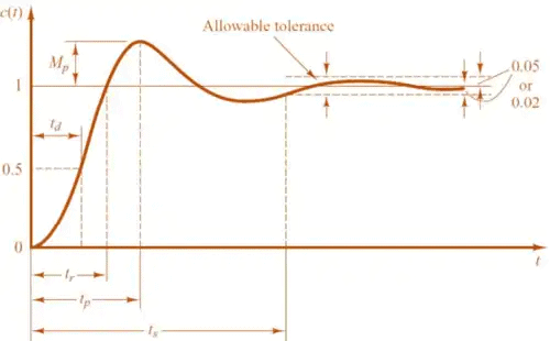
- Delay time (td): It is the time required for the response to reach 50% of the final value in first attempt.
The expression of delay time, td for second order system is: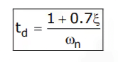
- Rise time, (tr): It is the time required for the response to rise from 0 to 100% of the final value for the under-damped system.
The expression of rise time, tr for second order system is: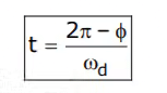
- Peak time, (tp): It is the time required for the response to reach the peak of time response or the peak overshoot.
The expression of peak time, tp for second order system is:
tP = nπ / ωd seconds
For first peak, n = 1 (maxima)
tP = π / ωd
For first minima, n = 2
tP = nπ / ωd
For second maxima, n = 3
tP = 3π / ωd - Settling time, (ts): It is the time required for the response to reach and stay within a specified tolerance band ( 2% or 5%) of its final value.
The expression of settling time, ts for second order system is:
For 2% tolerance band,
For 2% tolerance band,
- Peak overshoot (Mp): It is the normalized difference between the time response peak and the steady output and is defined as
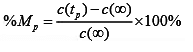
The expression of peak overshoot, Mp for second order system is: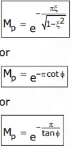
Where tanφ =
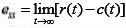
- Steady-state error (ess): It indicates the error between the actual output and desired output as ‘t’ tends to infinity.
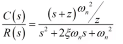
Effect of Adding a Zero to a System
If we add a zero at s = -z be added to a second order system. Then we have,
- The multiplication term is adjusted to make the steady-state gain of the system unity.
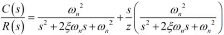
Manipulation of the above equation gives,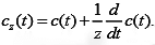
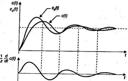
- The effect of added derivative term is to produce a pronounced early peak to the system response.
- Closer the zero to the origin, the more pronounce the peaking phenomenon.
- Due to this fact, the zeros on the real axis near the origin are generally avoided in design. However, in a sluggish system the artful introduction of a zero at the proper position can improve the transient response.
Types of Feedback Control System
The open-loop transfer function of a system can be written as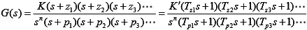
- If n = 0, the system is called type-0 system, if n = 1, the system is called type-1 system, if n = 2, the system is called type-2 system, etc.
Steady-State Error and Error Constants
The steady-state performance of a stable control system is generally judged by its steady-state error to step, ramp and parabolic inputs. For a unity feedback system,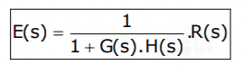
Where,
E(s) is error signal
R(s) is input signal
G(s) H(s) is the open loop transfer function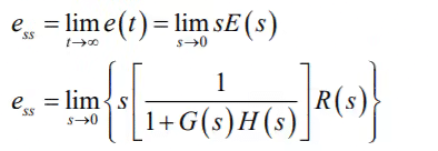
It is seen that steady-state error depends upon the input R(s) and the forward transfer function G(s).
- If input is unit step i.e R(t) = u(t)
R(s) = 1/s
Steady state error is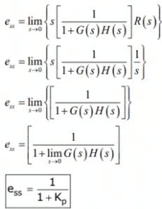
where,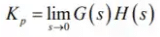
Kp is positional error constant. - If input is unit ramp i.e R(t) = tu(t)
R(s) = 1/s2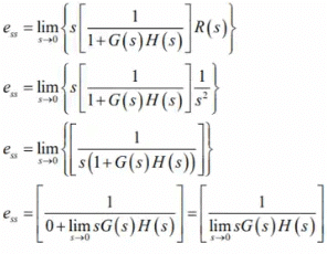
ess = 1/Kv
where,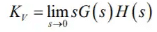
Kv is velocity error constant. - If input is unit parabolic i.e R(t) = 0.5tu(t)
R(s) = 1/s3
Steady state error,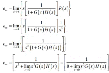
ess = 1/Ka
where,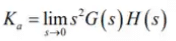
Ka is acceleration error constant.
The document Unit Impulse Response of 2nd Order System | Control Systems - Electrical Engineering (EE) is a part of the Electrical Engineering (EE) Course Control Systems.
All you need of Electrical Engineering (EE) at this link: Electrical Engineering (EE)
|
54 videos|83 docs|40 tests
|


FAQs on Unit Impulse Response of 2nd Order System - Control Systems - Electrical Engineering (EE)
| 1. What is a unit impulse response? |  |
| 2. How is the unit impulse response of a 2nd order system calculated? | |
Ans. The unit impulse response of a 2nd order system can be calculated by finding the inverse Laplace transform of the transfer function of the system. This involves manipulating the Laplace transform equation to isolate the impulse response and then applying the inverse Laplace transform to obtain the time-domain response.
| 3. What information can be obtained from the unit impulse response of a 2nd order system? | |
Ans. The unit impulse response of a 2nd order system provides insights into the system's stability, damping ratio, natural frequency, and overall response characteristics. It allows us to analyze how the system will behave when subjected to different input signals or disturbances.
| 4. How does the damping ratio affect the unit impulse response of a 2nd order system? | |
Ans. The damping ratio determines the shape and behavior of the unit impulse response of a 2nd order system. Higher damping ratios lead to overdamped responses, where the system takes longer to reach steady-state and exhibits less oscillation. Lower damping ratios result in underdamped responses, characterized by oscillations and a faster settling time.
| 5. Can the unit impulse response of a 2nd order system be used to determine the system's stability? | |
Ans. Yes, the unit impulse response can provide information about the stability of a 2nd order system. If the unit impulse response decays to zero over time, the system is considered stable. However, if the response grows indefinitely or exhibits oscillations, the system is unstable. By analyzing the shape and behavior of the unit impulse response, one can assess the stability of the system.
About this Document

4.95/5
Rating

Apr 13, 2025
Last updated
Document Description: Unit Impulse Response of 2nd Order System for Electrical Engineering (EE) 2025 is part of Control Systems preparation.
The notes and questions for Unit Impulse Response of 2nd Order System have been prepared according to the Electrical Engineering (EE) exam syllabus. Information about Unit Impulse Response of 2nd Order System covers topics
like and Unit Impulse Response of 2nd Order System Example, for Electrical Engineering (EE) 2025 Exam. Find important definitions, questions, notes, meanings, examples, exercises and tests below for Unit Impulse Response of 2nd Order System.
Introduction of Unit Impulse Response of 2nd Order System in English is available as part of our Control Systems
for Electrical Engineering (EE) & Unit Impulse Response of 2nd Order System in Hindi for Control Systems course.
Download more important topics related with notes, lectures and mock test series for Electrical Engineering (EE)
Exam by signing up for free. Electrical Engineering (EE): Unit Impulse Response of 2nd Order System | Control Systems - Electrical Engineering (EE)
Description
Full syllabus notes, lecture & questions for Unit Impulse Response of 2nd Order System | Control Systems - Electrical Engineering (EE) - Electrical Engineering (EE) | Plus excerises question with solution to help you revise complete syllabus for Control Systems | Best notes, free PDF download
Information about Unit Impulse Response of 2nd Order System
In this doc you can find the meaning of Unit Impulse Response of 2nd Order System defined & explained in the simplest way possible. Besides explaining types of
Unit Impulse Response of 2nd Order System theory, EduRev gives you an ample number of questions to practice Unit Impulse Response of 2nd Order System tests, examples and also practice Electrical Engineering (EE)
tests

Related Searches
MCQs
,past year papers
,video lectures
,shortcuts and tricks
,Unit Impulse Response of 2nd Order System | Control Systems - Electrical Engineering (EE)
,ppt
,Previous Year Questions with Solutions
,Summary
,Semester Notes
,Exam
,Free
,Viva Questions
,Extra Questions
,practice quizzes
,mock tests for examination
,Important questions
,Unit Impulse Response of 2nd Order System | Control Systems - Electrical Engineering (EE)
,Unit Impulse Response of 2nd Order System | Control Systems - Electrical Engineering (EE)
,study material
,Sample Paper
,Objective type Questions
;


Additional Information about Unit Impulse Response of 2nd Order System for Electrical Engineering (EE) Preparation
Unit Impulse Response of 2nd Order System Free PDF Download
The Unit Impulse Response of 2nd Order System is an invaluable resource that delves deep into the core of the Electrical Engineering (EE) exam.
These study notes are curated by experts and cover all the essential topics and concepts, making your preparation more efficient and effective.
With the help of these notes, you can grasp complex subjects quickly, revise important points easily,
and reinforce your understanding of key concepts. The study notes are presented in a concise and easy-to-understand manner,
allowing you to optimize your learning process. Whether you're looking for best-recommended books, sample papers, study material,
or toppers' notes, this PDF has got you covered. Download the Unit Impulse Response of 2nd Order System now and kickstart your journey towards success in the Electrical Engineering (EE) exam.
Importance of Unit Impulse Response of 2nd Order System
The importance of Unit Impulse Response of 2nd Order System cannot be overstated, especially for Electrical Engineering (EE) aspirants.
This document holds the key to success in the Electrical Engineering (EE) exam.
It offers a detailed understanding of the concept, providing invaluable insights into the topic.
By knowing the concepts well in advance, students can plan their preparation effectively.
Utilize this indispensable guide for a well-rounded preparation and achieve your desired results.
Unit Impulse Response of 2nd Order System Notes
Unit Impulse Response of 2nd Order System Notes offer in-depth insights into the specific topic to help you master it with ease.
This comprehensive document covers all aspects related to Unit Impulse Response of 2nd Order System.
It includes detailed information about the exam syllabus, recommended books, and study materials for a well-rounded preparation.
Practice papers and question papers enable you to assess your progress effectively.
Additionally, the paper analysis provides valuable tips for tackling the exam strategically.
Access to Toppers' notes gives you an edge in understanding complex concepts.
Whether you're a beginner or aiming for advanced proficiency, Unit Impulse Response of 2nd Order System Notes on EduRev are your ultimate resource for success.
Unit Impulse Response of 2nd Order System Electrical Engineering (EE) Questions
The "Unit Impulse Response of 2nd Order System Electrical Engineering (EE) Questions" guide is a valuable resource for all aspiring students preparing for the
Electrical Engineering (EE) exam. It focuses on providing a wide range of practice questions to help students gauge
their understanding of the exam topics. These questions cover the entire syllabus, ensuring comprehensive preparation.
The guide includes previous years' question papers for students to familiarize themselves with the exam's format and difficulty level.
Additionally, it offers subject-specific question banks, allowing students to focus on weak areas and improve their performance.
Study Unit Impulse Response of 2nd Order System on the App
Students of Electrical Engineering (EE) can study Unit Impulse Response of 2nd Order System alongwith tests & analysis from the EduRev app,
which will help them while preparing for their exam. Apart from the Unit Impulse Response of 2nd Order System,
students can also utilize the EduRev App for other study materials such as previous year question papers, syllabus, important questions, etc.
The EduRev App will make your learning easier as you can access it from anywhere you want.
The content of Unit Impulse Response of 2nd Order System is prepared as per the latest Electrical Engineering (EE) syllabus.
|
© EduRev
|
Education Revolution
|


|


Signup on EduRev and stay on top of your study goals
10M+ students crushing their study goals daily