State Space Representation of Control System | Control Systems - Electrical Engineering (EE) PDF Download

State Space Analysis
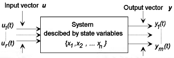
The so-called state-space description provide the dynamics as a set of coupled first-order differential equations in a set of internal variables known as state variables, together with a set of algebraic equations that combine the state variables into physical output variables.
State
The state of a dynamic system refers to a minimum set of variables, known as state variables, that fully describe the system.
- A mathematical description of the system in terms of a minimum set of variables, xi(t), i = 1,...,n, together with knowledge of those variables at an initial time t0, and the system inputs for time t ≥ t0, are sufficient to predict the future system state and outputs for all time t > t0.
- The dynamic behaviour of a state-determined system is completely characterized by the response of the set of n variables xi(t), where the number n is defined to be the order of the system.
- The system shown in the above figure has two inputs u1(t) and u2(t), and four output variables y1(t) ,..., y4(t). If the system is state-determined, knowledge of its state variables (x1(t0), x2(t0),...,xn(t0)) at some initial time t0, and the inputs u1(t) and u2(t) for t ≥ t0 is sufficient to determine all future behaviour of the system.
- The state variables are an internal description of the system which completely characterize the system state at any time t, and from which any output variables yi(t) may be computed.
The State Equations
In the standard mathematical form of the system is expressed as a set of n coupled first-order ordinary differential equations, known as the state equations, in which the time derivative of each state variable is expressed in terms of the state variables x1(t) ,..., xn(t) and the system inputs u1(t) ,..., ur(t). In the general case the form of the n state equations is:
x1 = f1(x, u, t)
x2 = f2(x, u, t)
xn = fn(x, u, t)
- where
 = dxi / dt and each of the functions fi (x, u, t), (i = 1,...,n) may be a general nonlinear, time varying function of the state variables, the system inputs, and time.
 - It is common to express the state equations in a vector form, in which the set of n state variables is written as a state vector x(t)=[x1(t), x2(t),...,xn(t)]T, and the set of r inputs is written as an input vector u(t)=[u1(t), u2(t),...,ur(t)]T. Each state variable is a time varying component of the column vector x(t).
- In vector notation the set of n equations in Eqs. (1) may be written
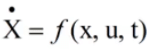
where f (x, u, t) is a vector function with n components fi (x, u, t).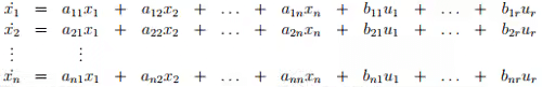
where the coefficients aij and bij are constants that describe the system.
Last equation can be written in matrix form as below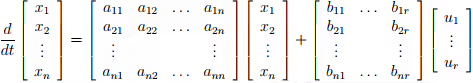
which may be summarized as: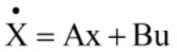
- Where state vector x is a column vector of length n, the input vector u is a column vector of length r, A is an n × n square matrix of the constant coefficients aij , and B is an n × r matrix of the coefficients bij that weight the inputs.
Output Equations
A system output is defined to be any system variable of interest. An arbitrary output variable in a system of order n with r inputs may be written as
y(t) = c1x1 + c2x2 + ... + cnxn + d1u1 + ... + drur
where the ci and di are constants. If a total of m system variables are defined as outputs, then the output equation can also be obtained as State Equation in compact form
y = Cx + Du
- where y is a column vector of the output variables yi(t), C is an m×n matrix of the constant coefficients cij that weight the state variables, and D is an m × r matrix of the constant coefficients dij that weight the system inputs.
- For many physical systems the matrix D is the null matrix, and the output equation reduces to a simple weighted combination of the state variable
if D= 0 ; then Y = Cx
Block Diagram Representation of Linear Systems Described by State Equations
A system of order n has n integrators in its block diagram. The derivatives of the state variables are the inputs to the integrator blocks, and each state equation expresses a derivative as a sum of weighted state variables and inputs. A detailed block diagram representing a system of order n may be constructed directly from the state and output equations as follows: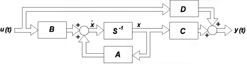
- Draw n integrator (S−1) blocks, and assign a state variable to the output of each block.
- At the input to each block (which represents the derivative of its state variable) draw a summing element.
- Use the state equations to connect the state variables and inputs to the summing elements through scaling operator blocks.
- Expand the output equations and sum the state variables and inputs through a set of scaling operators to form the components of the output.
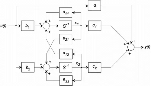
Example: Draw a block diagram for the general second-order, single-input single-output system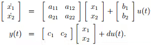
block diagram shown below is drawn using the four steps described above
Transformation from Classical Form to State-Space Representation
Let the differential equation representing the system be of order n, and without loss of generality assume that the order of the polynomial operators on both sides is the same.
(ansn + an−1sn−1+ ··· + a0)Y(s) =(bnsn + bn−1sn−1 + ··· + b0)U(s)
- We may multiply both sides of the equation by s−n to ensure that all differential operators have been eliminated
an + an − 1s−1 + ··· + a1s−(n−1) + a0s − nY(s) = bn + bn − 1s−1 + ··· + b1s−(n − 1)+ ··· + b0s−nU(s)
from which the output may be specified in terms of a transfer function. If we define a dummy variable Z(s), and split into two parts
Eq. of Z(s) can ne be solved for U(s)
U(s) = (an + an − 1s−1 + ··· + a1s−(n − 1) + a0s−nX(s)
State-Space and Transfer Function
The state equation form 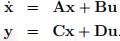 can be transformed into transfer function.
Tanking the Laplace transform and neglect initial condition then
sX(s) - X(0) = AX(s) + BU(s)
y(s) = CX(s) + DU(s)
then sX(s) - AX(s)= X(0) + BU(s)
By Neglecting Initial Conditions
(sI - A)X(s) = BU(s)
X(s) = (sI - A)-1 BU(s)
Then Put the value of X(s) for Y(s)...
then Y(s) = C(sI - A)-1BU(s) + DU(s)
Y(s) / U(s) = G(s) = C(sI - A)-1B + D
State-Transition Matrix
The state-transition matrix is defined as a matrix that satisfies the linear homogeneous state equation:
dx(t) / dt = Ax(t) ...(i)
Let ϕ(t) be the n × n matrix that represents the state-transition matrix; then it must satisfy the equation:
dϕ(t) / dt =Aϕ(t) ...(ii)
Furthermore, let x(0) denote the initial state at t = 0; then ϕ(t) is also defined by the matrix equation:
x(t) = ϕ(t) x (0) ...(iii)
which is the solution of the homogeneous state equation for t ≥ 0. One way of determining ϕ(t) is by taking the Laplace transform on both sides of Eq. (i); we have
s(X)(s) - x(0) = AX(s) ...(iv)
Solving for X(s) from Eq. (v). we get
X(s) = (SI - A)-1X(s) ...(v)
where it is assumed that the matrix (s1 – A) is non-singular. Taking the inverse Laplace transform on both sides of Eq. (v) yields
x(t) = L-1[(S1 - A)-1 x (0) t ≥ 0 ...(vi)
By comparing Eq.(iv) with Eq. (v), the state-transition matrix is identified to be
ϕ(t) = L-1[(sI - A)-1] ...(vii)
An alternative way of solving the homogeneous state equation is to assume a solution, as in the classical method of solving linear differential equations. We let the solution to be
x(t) = eATX(0)
for t ≥ 0, where eAt represents the following power series of the matrix At, and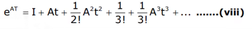
Properties of State-Transition Matrices.
The state-transition matrix OM possesses the following properties
- ϕ(0) = I (the identity matrix)
- ϕ-1(t) = ϕ(-t)
- ϕ(t2 - t1)ϕ(t1 - t0) = ϕ(t2 - t0) for any t0, t1, t2
- [ϕ(t)k = ϕ(kt) for k = positive integer
Controllability & Observability
1. Controllability: Controllability can be define in order to be able to do whatever we want with the given dynamic system under control input, the system must be controllable. A system is said to be controllable at time t0 if it is possible by means of an unconstrained control vector to transfer the system from any initial state to any other state in a finite interval of time.
Condition for Controllability;
If the rank of CB = [ B : AB : ..... An - 1B is equal to n ], then the system is controllable.
2. Observability: In order to see what is going on inside the system under observation, the system must be observable. A system is said to be observable at time t0 if, with the system in state X(t0),it is possible to determine this state from the observation of the output over a finite interval of time.
Condition for Observability: If the rank of OB = [ CT : ATCT : ..... AT)n - 1CT is equal to n], then the system is sail to be Observable.
|
53 videos|107 docs|40 tests
|
FAQs on State Space Representation of Control System - Control Systems - Electrical Engineering (EE)
| 1. What is state space analysis in control systems? |  |
| 2. How is a control system represented in state space form? | |
| 3. What are the advantages of using state space analysis in control systems? | |
| 4. How does state space analysis differ from transfer function analysis? | |
| 5. How can state space analysis be used in practical control system design? | |


Viva Questions
,mock tests for examination
,past year papers
,Previous Year Questions with Solutions
,study material
,State Space Representation of Control System | Control Systems - Electrical Engineering (EE)
,Objective type Questions
,Summary
,Important questions
,shortcuts and tricks
,State Space Representation of Control System | Control Systems - Electrical Engineering (EE)
,Sample Paper
,practice quizzes
,MCQs
,Exam
,Free
,ppt
,Extra Questions
,State Space Representation of Control System | Control Systems - Electrical Engineering (EE)
,video lectures
,Semester Notes
;


State Space Representation of Control System Free PDF Download
Importance of State Space Representation of Control System
State Space Representation of Control System Notes
State Space Representation of Control System Electrical Engineering (EE) Questions
Study State Space Representation of Control System on the App
|
© EduRev
|
Education Revolution
|


|


