Mathematical Models | Control Systems - Electrical Engineering (EE) PDF Download

Introduction

The control systems can be represented with a set of mathematical equations known as mathematical model. These models are useful for analysis and design of control systems. Analysis of control system means finding the output when we know the input and mathematical model. Design of control system means finding the mathematical model when we know the input and the output.

The following mathematical models are mostly used.

• Differential equation model
• Transfer function model
• State space model

Differential Equation Model

Differential equation model is a time domain mathematical model of control systems. Follow these steps for differential equation model.

• Apply basic laws to the given control system.
• Get the differential equation in terms of input and output by eliminating the intermediate variable(s).

Example:

Consider the following electrical system as shown in the following figure. This circuit consists of resistor, inductor and capacitor. All these electrical elements are connected in series. The input voltage applied to this circuit is vi and the voltage across the capacitor is the output voltage vo.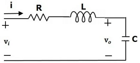

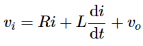
• Mesh equation for this circuit is
  
• Substitute, the current passing through capacitorin the above equation.
  
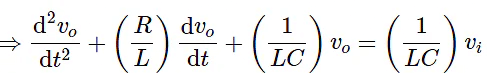
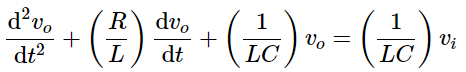
• The above equation is a second order differential equation.

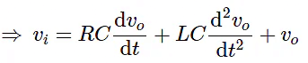
Transfer Function Model

Transfer function model is an s-domain mathematical model of control systems. The Transfer function of a Linear Time Invariant (LTI) system is defined as the ratio of Laplace transform of output and Laplace transform of input by assuming all the initial conditions are zero.

• If x(t) and y(t) are the input and output of an LTI system, then the corresponding Laplace transforms are X(s) and Y(s).
• Therefore, the transfer function of LTI system is equal to the ratio of Y(s) and X(s).
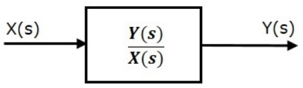
  i.e., Transfer Function = Y(s)/X(s)
• The transfer function model of an LTI system is shown in the following figure.
  
• Here, we represented an LTI system with a block having transfer function inside it. And this block has an input X(s) & output Y(s).

Example:

• Previously, we got the differential equation of an electrical system as
  
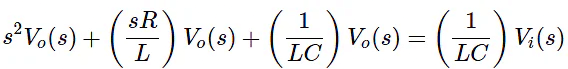
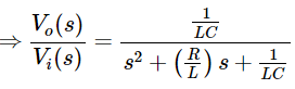
• Apply Laplace transform on both sides.
  
• Where,
  • v_i(s) is the Laplace transform of the input voltage v_i
  • v_o(s) is the Laplace transform of the output voltage v_o
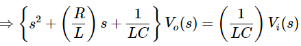
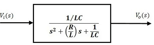
• The above equation is a transfer function of the second order electrical system. The transfer function model of this system is shown below.
  
• Here, we show a second order electrical system with a block having the transfer function inside it. And this block has an input V_i(s) & an output V_o(s).

• State Space Model

  The State Space Model is a time-domain mathematical model used to describe a system. It represents the system with a set of first-order differential equations that express the dynamics of the system in terms of state variables. The state-space representation is particularly useful for analyzing and designing modern control systems.

  Steps for State Space Model:

  1. Define State Variables:

     • Choose state variables that represent the internal conditions of the system. For electrical systems, these can often be voltages and currents.
     • Let the state variables be denoted by x(t) (a vector) and the output be denoted by y(t).

  2. Formulate the State Equations:

     • The state equations describe the relationship between the input and the state variables.
     • These are written in the form: $$\frac{d}{dt} \mathbf{x}(t) = A\mathbf{x}(t) + B\mathbf{u}(t)$$dtdx(t)=Ax(t)+Bu(t) where:
       • x(t) is the state vector (containing the state variables).
       • u(t) is the input vector.
       • A is the system matrix (describes the system dynamics).
       • B is the input matrix (describes how the input affects the state variables).

  3. Formulate the Output Equation:

     • The output equation describes the relationship between the output and the state variables.
     • This is written in the form: $$\mathbf{y}(t) = C\mathbf{x}(t) + D\mathbf{u}(t)$$y(t)=Cx(t)+Du(t) where:
       • y(t) is the output vector.
       • C is the output matrix (describes how the state variables contribute to the output).
       • D is the feedthrough matrix (describes how the input directly affects the output).

  Example:

  Consider the same second-order electrical system with resistor R, inductor L, and capacitor C connected in series. The input is the voltage applied to the circuit v_i(t), and the output is the voltage across the capacitor v_o(t).

  1. State Variables:

     • Let the state variables be:
       • x₁(t) = i(t) (current through the circuit)
       • x₂(t) = v_o(t) (voltage across the capacitor)

  2. State Equations:

     • Using Kirchhoff's Voltage Law (KVL) and the relationships for resistors, inductors, and capacitors, we derive the state equations.

     From the electrical system, the equations are:

     $$L \frac{d}{dt} i(t) + Ri(t) + v_o(t) = v_i(t)$$Ldtdi(t)+Ri(t)+vo(t)=vi(t)$$C \frac{d}{dt} v_o(t) = i(t)$$Cdtdvo(t)=i(t)

     These can be written in the matrix form:

     $$\frac{d}{dt} \begin{bmatrix} x_1(t) \\ x_2(t) \end{bmatrix} = \begin{bmatrix} -\frac{R}{L} & -\frac{1}{L} \\ \frac{1}{C} & 0 \end{bmatrix} \begin{bmatrix} x_1(t) \\ x_2(t) \end{bmatrix} + \begin{bmatrix} \frac{1}{L} \\ 0 \end{bmatrix} v_i(t)$$dtd[x1(t)x2(t)]=[−LRC1−L10][x1(t)x2(t)]+[L10]vi(t)

  3. Output Equation:

     • The output is the voltage across the capacitor, i.e., y(t) = v_o(t) = x₂(t).

     Thus, the output equation is:

     $$y(t) = \begin{bmatrix} 0 & 1 \end{bmatrix} \begin{bmatrix} x_1(t) \\ x_2(t) \end{bmatrix} + \begin{bmatrix} 0 \end{bmatrix} v_i(t)$$y(t)=[01][x1(t)x2(t)]+[0]vi(t)

  Final State-Space Representation:

  The state-space model for the system is:

  $$\frac{d}{dt} \begin{bmatrix} x_1(t) \\ x_2(t) \end{bmatrix} = \begin{bmatrix} -\frac{R}{L} & -\frac{1}{L} \\ \frac{1}{C} & 0 \end{bmatrix} \begin{bmatrix} x_1(t) \\ x_2(t) \end{bmatrix} + \begin{bmatrix} \frac{1}{L} \\ 0 \end{bmatrix} v_i(t)$$dtd[x1(t)x2(t)]=[−LRC1−L10][x1(t)x2(t)]+[L10]vi(t)$$y(t) = \begin{bmatrix} 0 & 1 \end{bmatrix} \begin{bmatrix} x_1(t) \\ x_2(t) \end{bmatrix}$$y(t)=[01][x1(t)x2(t)]

  Here:

  • A = $\begin{bmatrix} -\frac{R}{L} & -\frac{1}{L} \\ \frac{1}{C} & 0 \end{bmatrix}$[−LRC1−L10]
  • B = $\begin{bmatrix} \frac{1}{L} \\ 0 \end{bmatrix}$[L10]
  • C = $\begin{bmatrix} 0 & 1 \end{bmatrix}$[01]
  • D = $\begin{bmatrix} 0 \end{bmatrix}$[0]

  This state-space representation provides a systematic way to analyze and design control systems, especially when dealing with multiple state variables and non-linear systems.