Transient & Steady State Analysis of Linear Time Invariant (LTI) Systems | Control Systems - Electrical Engineering (EE) PDF Download

Time Response Analysis
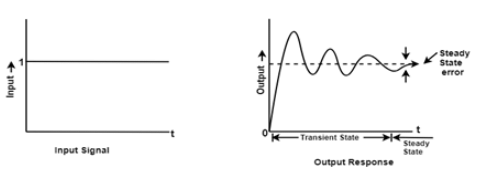
When the energy state of any system is disturbed, and the disturbances occur at input, output or both ends, then it takes some time to change from one state to another state. This time that is required to change from one state to another state is known as transient time and the value of current and voltage during this period is called transient response.
Depending upon the parameters of the system, the transient may have oscillations which may be either sustained or decaying in nature.
Thus time response of a control system is divided into two parts-
- Transient response analysis.
- Steady State Analysis.
Transient State Response
It deals with the nature of the response of a system when subjected to an input.
Steady State Analysis
It deals with the estimation of the magnitude of steady-state error between input and output.
Different Type of Standard Test Signals
The various inputs or disturbances affecting the performance of a system are mathematically represented as a standard test signal.
- Step signal ( sudden input )
- Ramp Signal (velocity type of input )
- Parabolic Signal ( type of acceleration input )
- Impulse signal (sudden shock )
Note
- Step signal and impulse signal are bounded input signal.
- Ramp signal and parabolic signal are an unbounded input signal.
- Step signal, a ramp signal, and periodic signal are for time domain analysis. Only an impulse signal is essential for steady-state analysis.
Characteristics of Time-domain Analysis
- Every transfer function representing the control system is of a particular type of order.
- The steady state analysis depends upon the type of the system.
- The type of the system is determined from open loop transfer function G(S).H(S)
Transient Time: The time required to change from one state to another is called the transient time.
Transient Response: The value of current and voltage during the time change is called transient response.
Transient and Steady State Analysis of Linear Time Invariant (LTI) Systems
So, we can say that the transient response is the part of the response which goes to zero as time increases and the steady-state response is the part of the total response after transient has died. If the steady-state response is the part of the output does not match with the input then the system has a steady state error.
Test Input Signal for Transient Analysis
For the analysis of the time response of a control system, the following input signals are used.
(a) Step Function
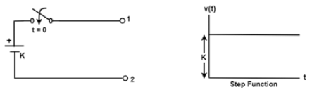
A unit step function is denoted by u(t) and is defined as
u(t) = 0 ; t=0
= 1 ;0=t
Laplace Transform
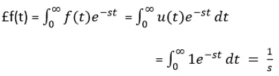
Step function is also called displacement function. If input is R(S), then R(s) = 1/s
Example: Imagine turning on a light switch. At t=0, the light goes from off (0) to on (1) instantly. This transition can be represented by the unit step function.
(b) Ramp Function
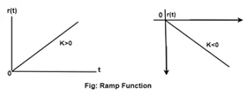
This function starts from the origin and linearly decreases or increases with time as shown in the figure above.
Let r(t) be the ramp function then
r(t) = 0 ; t<0
= Kt ; t>0
Where 'K' is the slope of the line, for a positive value of 'K' the slope is upward, and the slope is downward for the negative value of 'K.'
Laplace transform
Example: Think of a car accelerating uniformly from a standstill. The speed of the car increases linearly with time, which can be represented by the ramp function.
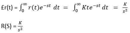
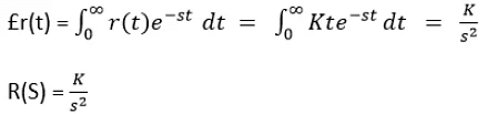
(c) Parabolic Function
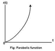
The value of r(t) is zero when t<0 and is a quadratic function of time when t>0.
Therefore r(t) = 0 ; t<0
= (Kt2)/2 ; t>0
Where 'K' is constant for unit parabolic function K = 1. The unit parabolic function is defined as
r (t) = 0 ; t<0
= t2/2 ; t>0
Laplace Transform
Example: Imagine an object in free fall under gravity. The distance it falls is proportional to the square of the time. This relationship can be represented by the parabolic function.
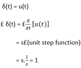
(d) Impulse Function

A unit impulse function is defined as
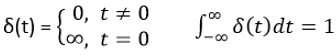
Thus we can say that impulse function has zero value everywhere except at t=0 where the amplitude is infinite.
Example: A quick, intense pulse of light or an electrical spike can be modeled using the impulse function.
|
53 videos|107 docs|40 tests
|
FAQs on Transient & Steady State Analysis of Linear Time Invariant (LTI) Systems - Control Systems - Electrical Engineering (EE)
| 1. What is time response analysis in the context of electrical engineering? |  |
| 2. What is the purpose of transient analysis in time response analysis? | |
| 3. What does steady-state analysis involve in time response analysis? | |
| 4. How are linear time-invariant (LTI) systems relevant in time response analysis? | |
| 5. What are some commonly used input signals in transient analysis for time response analysis? | |


Exam
,Extra Questions
,Semester Notes
,Free
,Objective type Questions
,Sample Paper
,ppt
,practice quizzes
,past year papers
,shortcuts and tricks
,MCQs
,Viva Questions
,study material
,Transient & Steady State Analysis of Linear Time Invariant (LTI) Systems | Control Systems - Electrical Engineering (EE)
,Previous Year Questions with Solutions
,mock tests for examination
,video lectures
,Important questions
,Transient & Steady State Analysis of Linear Time Invariant (LTI) Systems | Control Systems - Electrical Engineering (EE)
,Summary
,Transient & Steady State Analysis of Linear Time Invariant (LTI) Systems | Control Systems - Electrical Engineering (EE)
;


Transient & Steady State Analysis of Linear Time Invariant (LTI) Systems Free PDF Download
Importance of Transient & Steady State Analysis of Linear Time Invariant (LTI) Systems
Transient & Steady State Analysis of Linear Time Invariant (LTI) Systems Notes
Transient & Steady State Analysis of Linear Time Invariant (LTI) Systems Electrical Engineering (EE) Questions
Study Transient & Steady State Analysis of Linear Time Invariant (LTI) Systems on the App
|
© EduRev
|
Education Revolution
|


|


