Time Response of First Order System | Control Systems - Electrical Engineering (EE) PDF Download

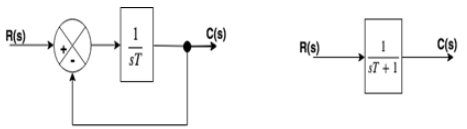
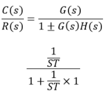
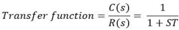
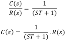
In the above transfer function, the power of 's' is the one in the denominator. That is why the above transfer function is of the first order, and the system is said to be the first order system.
Response of 1st order system when the input is unit step -
For Unit Step,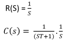
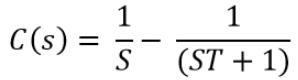
Now, the partial fraction of above equation will be: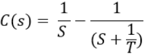
Taking the inverse Laplace of above equation is: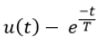
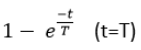
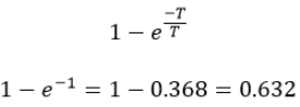
Where T is known as time constant of the system and it is defined as the time required for the signal to attain 63.2 % of final or steady state value. Time constant means how fast the system reaches the final value. As smaller the time constant, as faster is the system response. If time constant is larger, system goes to move slow.
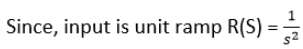
Time response of first order system with unit ramp signal is -
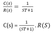
Now, putting the value of R(S) in the equation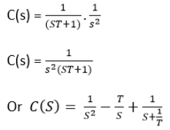
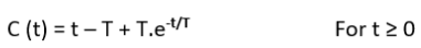
Now taking the inverse Laplace of the above equation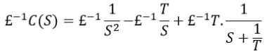
The error signal e(t) will be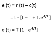
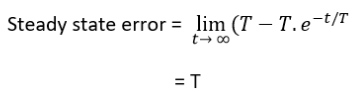
The steady state error is equal to 'T,' where 'T' is the time constant of the system. For a small time constant, the error is small, and the response of the system increases.
Response of 1st order system with unit impulse function is -
Value of impulse = 1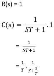
Inverse Laplace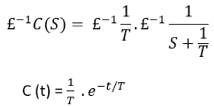
|
53 videos|107 docs|40 tests
|


Semester Notes
,Extra Questions
,Objective type Questions
,Sample Paper
,practice quizzes
,ppt
,mock tests for examination
,Free
,Time Response of First Order System | Control Systems - Electrical Engineering (EE)
,Time Response of First Order System | Control Systems - Electrical Engineering (EE)
,MCQs
,study material
,Summary
,shortcuts and tricks
,Previous Year Questions with Solutions
,Exam
,Viva Questions
,Important questions
,past year papers
,Time Response of First Order System | Control Systems - Electrical Engineering (EE)
,video lectures
;


Time Response of First Order System Free PDF Download
Importance of Time Response of First Order System
Time Response of First Order System Notes
Time Response of First Order System Electrical Engineering (EE) Questions
Study Time Response of First Order System on the App
|
© EduRev
|
Education Revolution
|


|


within 7 days!