Bode Plot | Control Systems - Electrical Engineering (EE) PDF Download

Introduction

• It is a frequency response plot that contains two graphs, magnitude and phase. The first plot is the magnitude plot of sinusoidal transfer function versus log ω, and the other graph represents the phase angle. It can be drawn both for the open-loop and closed-loop system. It is generally drawn for the open-loop system because it conveniently determines the stability and other related parameters.
• Bode plot helps us determine the system's stability and provides us with a way to improve that stability. The standard representation of the Bode plot of the open-loop system is given by:
  20 log|G(jω)|
• It represents the logarithmic magnitude of the function G(s) or G(jω). Here, the base of logarithmic is 10. The unit represents the magnitude of the logarithmic function G(jω) in decibels or db. The curve is not drawn on a simple graph paper; and instead, it is drawn on the semilog paper that uses the frequency, phase angle, and magnitude for plotting. The log scale or abscissa is used for the frequency, and the linear scale or ordinate for the phase angle and magnitude.
• The logarithmic function allows the various values in the forms of multiple to be added. For example,
  log ab = log a + log b
• Thus, the bode plot has an advantage of converting the multiplication of magnitudes in addition. For example,
  Let G(jω) = K/ jω (1 + jωT)
• The magnitude of G(jω) is K/[ ω (1 + ω² T²)^1/2]
• The phase angle of G(jω) is -90 - tan^-1ωT
• The magnitude in the form of decibels can be expressed as:
  20 log [K/ ω (1 + ω² T²)^1/2]
  = 20 log K/ ω + 20 log 1/(1 + ω² T²)^1/2
  = 20 log K/ ω - 20 log (1 + ω² T²)^1/2
• We have inserted the negative sign due to the inverse of the logarithmic value.
• It means that log 1/a can be written as log (a)^-1, which is equal to -log a.
• Thus, the above equation depicts that the magnitude when expressed in terms of db. It can easily convert the multiplicative terms to add, meaning that the individual factors of the given transfer function can be added. We will also discuss an example to draw a bode plot later in the topic.

Constant gain K in Bode plot

• The constant gain is represented by K. It is also known as the system gain in case of root locus and transfer functions.
  Let, G(s) = K
  G(s) = G(jω) = K
• The angle assumed for the constant gain is 0 degrees.
• In terms of decibels, we can represent the system gain as:
  A = |G(jω)| = 20log K
• If the value of K is negative, the angle thus will be 180 degrees.
  At the magnitude of the 20log K, the magnitude of constant gain K will be a horizontal straight line.
• There are three range of K.
  • K > 1
  • K = 1
  • 0 < K < 1
• When the value of K is greater than 1, 20log K is positive.
• When the value of K is 1, 20log K is zero. It is because the value of log 1 is 0.
• When the value of K is greater than 0 and less than 1, 20log K is negative.

Integral factor in Bode plot

• Both the integral factor and the derivative factor affect the slope of the magnitude curve. Let's first discuss the integral factor in the Bode plot.
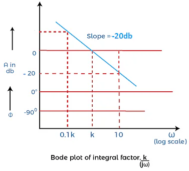
• Let the integral factor be K/ jω. The integral factor is represented by constant gain divided by the s, and it can be of one order or more.
  G(s) = K/s
  G(s) = K/ jω
• Its magnitude and phase angles are K/ω and -90 degrees.
• Its gain in decibels = A = |G(jω)| = 20log (K/ω)
• When ω = 0.1 K, A = 20log (K/0.1K) = 20log (10) = 20 db
• It is because the value of log 10 is 1.
• When ω = K, A = 20log (K/K) = 20log (1) = 0 db
• When ω = 10 K, A = 20log (K/10K) = 20log (10)^-1 = -20 db
• It is because the value of log a^-n is -n loga.
• From the above analysis for different values of ω, we can find the magnitude of the integral factor. It will be a straight line with a slope of -20 db. It will also pass through 0 db, when the value of ω is K.
• The plot of an integral factor K/ jω is shown below:
  
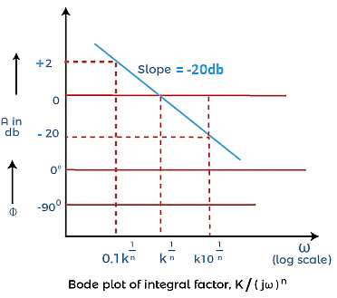
• Let's consider another example of an integral factor in the multiples of n. It is given by:
  G(s) = K/sⁿ
  G(s) = K/ jωⁿ
• Its magnitude and phase angle are K/ωⁿ and -90n degrees.
  Its gain in decibels = A = |G(jω)| = 20log (K/ωⁿ)
• The plot of an integral factor in the multiples of n is shown below:
  

Derivative factor in the Bode plot

• The derivative factor consists of the terms containing s in the numerator itself. Let's consider a derivative factor represented by K jω.
  G(s) = Ks = K jω
• Its magnitude and phase angles are Kω and 90 degrees.
• It is because the term jω is in the numerator. Thus, the angle will be in positive degrees.
• Its gain in decibels = A = |G(jω)| = 20log (Kω)
• When ω = 0.1/K, A = 20log (K x 0.1/K) = 20log (0.1) = 20log (10)^-1 = -20 db
• It is because the value of log a^-n is -n loga.
• When ω = 1/K, A = 20log (K/K) = 20log (1) = 0 db
• When ω = 10/ K, A = 20log (K x 10/ K) = 20log (10) = 20 db
• The plot of the above derivative factor is shown below:
  
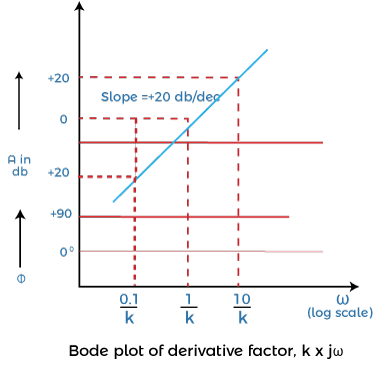
• It is because the value of log 10 is 1.
• From the above analysis for different values of ω, we can find the magnitude of the derivative factor. It will be a straight line with a slope of +20 db. It will also pass through 0 db, when the value of ω is 1/K.
• Let's consider another example of a derivative factor in the multiples of n. It is given by:
  G(s) = Ksn
  G(s) = Kjωn
• Its magnitude and phase angle are Kωn and 90n degrees.
• Its gain in decibels = A = |G(jω)| = 20log (Kωn)

First order factor in the numerator

• The first order factor in the numerator or a derivative factor is given by:
  G(s) = 1 + sT
  G(jω) = 1 + jωT
  |G(jω)| = (1 + ω² T²)1/2
  Angle = ?tan^-1ωT
• The gain in decibels is given by:
  A =20 log (1 + ω² T²)1/2
• The value of gain at very low frequencies (<<1) will be equal to 20 log 1 = 0 dB.
• The value of gain at high frequencies (>>1) will be equal to 20 log ωT.
• The Bode plot for the first order function given above is shown below:
  

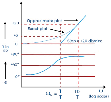
• We have approximated the magnitude of the plot in two straight lines. The first line is a straight horizontal line with very low frequencies (0 db), while the other slanting slope refers to the high frequencies (20 log ωT). It would have a slope of +20db.The two straight lines are the asymptotes of the exact curve. The frequency at which these two asymptotes meet is known as the corner frequency, and it is also known as break frequency.

• For the above-given function, the corner frequency will arise when ω = 1/T. The phase angle will vary from 0 degrees to 90 degrees with frequency variation between zero and infinity.
• The magnitude approximated at the corner frequency is around + 3dB, and it is generally considered the loss in db at this corner frequency.

First order factor in the denominator

• The first order factor in the denominator or an integral factor is given by:
  G(s) = 1/1 + sT
  G(jω) =1/ 1 + jωT
  |G(jω)| =1/ (1 + ω² T²)^1/2
  Angle = ?-tan^-1ωT
• The gain in decibels is given by:
  A = 20 log 1/(1 + ω² T²)^1/2
  A = 20 log (1 + ω² T²)^-1/2
  A = -20 log (1 + ω² T²)^1/2
• It is because the value of log a^-n is -n loga.
• The value of gain at very low frequencies (<<1) will be equal to -20 log 1 = 0 dB.
• The value of gain at high frequencies (>>1) will be equal to -20 log ωT.
• The Bode plot for the first order function given above is shown below:
  
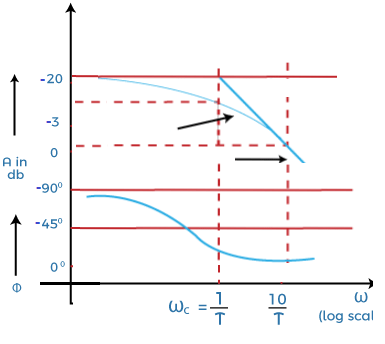
• We have approximated the magnitude of the plot in two straight lines. The first line is a straight horizontal line with the very low frequencies (0 db), while the other slanting slope refers to the high frequencies (-20 log T). It would have a slope of -20db.

Note: The derivative factor in the transfer function generally represents to the positive slope, while the integral factor represents the negative slope in the bode plot.

The two straight lines are the asymptotes of the exact curve. For the above-given function, the corner frequency will arise when ω = 1/T. The corner frequency divides the curve of the Bode plot into two regions, i.e., low frequency and high frequency. The phase angle will vary from 0 degrees to -90 degrees with frequency variation between zero and infinity. The magnitude approximated at the corner frequency is around - 3dB, and it is generally considered the loss in db at this corner frequency.

Note: The two curves in the Bode plot is the magnitude curve and the phase angle curve. The first curve that represents the value in decibels represents the magnitude curve, while the second curve represents the phase angle curve.

Quadratic factor in the denominator

• It is the essential part of the Bode plot to understand. It means the factor in the denominator in present in the form of quadratic equation.
• Let's consider a quadratic equation, which is given by:
  G(s) = ω_n²/(s² + 2a ω_ns + ω_n²)
• Where,
  a is the damping ratio
  ω_n is the natural frequency
• We can write the above transfer function as:
  G(s) = 1/ (1 + 2as/ ω_n + (s/ ω_n)²
  Put, s = jω
  G(jω) = 1/ (1 + 2a jω/ ω_n + (jω / ω_n)²
  G(jω) = 1/(1 - (ω / ω_n)² + j²a ω/ ω_n
• The magnitude is given by:
  |G(jω) |= 1/[(1 - (ω / ω_n)4) + 4a² ω²/ ω_n²]^1/2
• The phase angle is given by:
  Angle G(jω) = tan^-1[(2a jω/ω_n)/(1 - (ω / ω_n)²)
• Let's find the gain of the above transfer function in decibels.
  A = 20log G(jω)
  A = 20 log 1/[(1 - (ω / ω_n)⁴ )+ 4a² ω²/ ωn²]^1/2
• The factor G(jω) is present in the denominator. To bring it in numerator, we will insert a negative sign. It is because log (1/a) is equal to -log a.
• So, the gain will be:
  A = -20 log [(1 - (ω / ω_n)⁴)+ 4a² ω²/ ω_n²]^1/2
• Let's find the value of gain at different frequencies.
• The value of gain at very low frequencies (ω<< ω_n) is equal to:
  A = -20 log [(1 - (ω² / ω_n²(2 - 4a²)+ ω⁴/ ω_n⁴]^1/2
  A = -20 log 1 = 0
• The value of gain at very high frequencies (ω>> ω_n) is equal to:
  A = -20 log [(1 - (ω² / ω_n²(2 - 4a²)+ ω⁴/ ω_n⁴]^1/2
  A = -20 log [ω⁴/ ω_n⁴]^1/2
  A = -20 log ω² / ω_n²
  A = -20 log [ω/ ω_n]²
• We know that log a² = 2 log a
  A = -20 x 2log [ω/ ω_n]
  A = -40 log [ω/ ω_n]
  At, ω = ω_n
  A = -40 log 1 = 0 db
  At, ω = 100ω_n
  A = -40 log 100
  A = -40 log 10²
  A = -40 x 2 log 10
  A = -80 log 10 = -80 db
  At, ω= 10ω_n
  A = -40 log 10 = -40
• Thus we can conclude that the magnitude plot of the quadratic factor can be approximated by two straight lines with a scale of 0 db and -40 db.
• Let' find the value of angle G(jω) at different values of frequency.
  Angle G(jω) = tan^-1[(2a jω/ω_n)/(1 - (ω / ωn)²)
  At, ω = ω_n
  Angle G(jω) = tan^-1(2a/0) = -90 degrees.
• It is because the value of tan^-1(infinity) is -90 degrees.
  At ω = 0, the value of angle is 0
  At ω = infinity, the value of angle tends to -180 degrees.
• The plot of the quadratic factor is denominator is shown below:
  
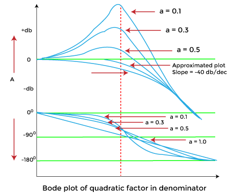
• The two curves are independent of the damping ratio a. The height of the resonant peak is inversely proportional to the damping ratio. It means that the decrease in the value of the damping ratio will increase the resonant peak.

Procedure to draw the magnitude curve and phase angle curve of the bode plot

Before proceeding, let's discuss the main conclusions obtained from the topic discussed above.

• The constant gain K, derivative, and integral factor in the bode plot contributes gain at all the frequencies.
• The higher order (two and more) factors in the transfer function contribute gain only when the frequency is greater than the corner frequency. The natural frequency in case of quadratic factor is assumed as corner frequency.

Let's discuss the steps that will help us to draw the bode plot.

• Convert the given transfer function into the time constant form, which is as follows: It helps us to easily find the corner frequencies.
• Arrange the corner frequencies in the increasing order. The format of the table is shown below:
  
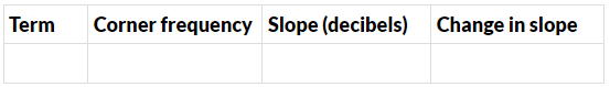
• The 'Term' specifies the separate constant gain, derivative factor, and the integral factor, such as, K, K/jω, or K (jω). The 'change in slope' includes the change in the value of the slope at each corer frequency.
• Select a frequency, which has the lower value compared to the lowest corner frequency. Now, calculate the value of the terms at that selected frequency.
• Find the gain in decibels one by one at every corner frequency. The formula to find the gain is given by:
  
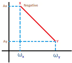
• Gain at ωy = (Slope from ωx to ωy x log ωy/ωx] + gain at ωx
• The frequencies ωx and ωy are shown below:
• Bode plot
• Now, we will perform step 4 again at a different frequency, which is greater than the highest corner frequency.
• Take a semilog graph paper and first mark the dimension on the axis to draw the plot. The magnitude will appear on the y-axis and the frequency range will appear on the x-axis.
• Mark the points calculated in the above steps on the semilog graph paper and join the points. The points on the graph paper should be joined only with straight lines. We can also mark the slope at every point on the graph.
• The plot is assumed as the approximated plot. The exact plot requires the exact calculation at every corner frequency.

Consider an example.
Let the transfer function be G(s) = K (1 + sT₁)²/s²(1 + sT₂)( 1 + sT₃)
Put, s = jω
G(jω) = K (1 + jω T₁)²/( jω)²(1 + jωT₂)( 1 + jωT₃)
The value of T1, T2, 3 in the increasing order will be T2 < T3 < T1.
There will be three corner frequencies at 1/T1, 1/T2, and 1/T3.
In the given transfer function G(s) = K (1 + sT₁)²/s²(1 + sT₂)( 1 + sT₃), there are four terms. Thus, we will first draw the magnitude plot of these four independent terms. The four terms are K/ jω , K(1 + sT₁), 1/(1 + sT₂), and 1/( 1 + sT₃). The first, third, and the fourth term represent the integral term with the slope of -20db. The second term is the derivative term that represents the positive slope.
The final plot will be the combined plot of all the four plots, as shown below: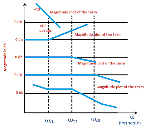
The above Bode plot shows that the first two terms have a slope of 40, while the other two has a slope of 20. The first two terms are in the form of squares in the transfer function, where log a2 is always equal to '2 log a.' Thus, it will appear with a slope of 40. As discussed above, the negative and positive terms with the slope are due to the integral and derivative factors.
Let's discuss how the value is combined.
A particular value at a region will be the result of the combined values at the above four sections. For example, the section between ωc1 and ωc3 will have the value by adding all section values (-40db + 40db + 0 + 0 = 0db).

Phase Margin and Gain Margin of a Bode Plot

• The phase angle is calculated at various values of frequency. The frequencies are generally the same frequencies selected for plotting the magnitude section of a Bode plot. The phase and magnitude sections are drawn in a single semilog sheet with a common frequency scale for easy plotting. It also saves time.

The relation between the phase margin and the phase angle is given by:
Y = 180 + a
Where,
Y is the phase margin
a is the phase angle
It is calculated at the gain crossover frequency.
If the phase cross over frequency is negative, the gain margin of the system is positive. Similarly, if the phase cross over frequency is positive, the gain margin of the system is negative.

Example: Sketch the Bode plot of the following transfer function G(s) = Ks²/(1 + 0.2s)(1 + 0.02s). Also determine the system gain K and the gain crossover frequency to be 5 radians/second.

G(s) = Ks²/(1 + 0.2s)(1 + 0.02s)

Step 1: Finding the corner frequencies
Here, we will first find the value of G(jω).
G(jω) = K j2ω2/(1 + 0.2jω)(1 + 0.02jω)
There will be two corner frequencies at T1 and T2, which are 0.2 and 0.02.
Thus, the corner frequencies are 1/0.2 = 5 radians/second and 1/0.02 = 50 radians/second.

Step 2: Preparing the table
As discussed in the above steps, we will prepare a table. There are three independent factors, j²ω², 1/(1 + 0.2jω), and 1/(1 + 0.02jω). So, the table will include three terms, as shown below:

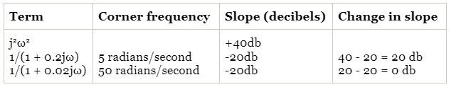
The first term will have a slope of 40 due to its square. The change in slope will include the sum of the slope from the top to bottom. The first row will have no change in the slope due to no term above it.

Step 3: We will find a frequency lower than the first corner frequency + a frequency higher than the second corner frequency.
The gain A = |G(jω)| = 20 log | j²ω²|
We will find the value of gain at selected low frequency, two corner frequencies, and the high frequency.
Let's select the frequency 0.5, which is lower than the first corner frequency.

• At, ω = low frequency, the value of gain is:
  A = |G(jω)| = 20 log | j²ω²|
  A = 20 log | 0.5²|
  A = 20 log 0.25
  A = 12 db
• At, ω = first corner frequency (5 db), the value of gain is:
  A = |G(jω)| = 20 log | j²ω²|
  A = 20 log | 5²|
  A = 20 log 25 or 40 log 5
  A = 28 db
• Now, at the second corner frequency and the selected higher corner frequency, we will use the formula:
  Gain at ω_y = (Slope from ωx to ωy x log ωy/ωx] + gain at ωx
  At ω_c2 = (Slope from ω_c1 to ω_c2 x log ω_c2/ω_c1] + gain at ω (ω = ω_c1)
  Where,
  ω_c1 = first corner frequency
  ω_c2 = second corner frequency
  Slope from ω_c1 to ω_c2 = change in slope of the second row
• At, ω = second corner frequency (50 db), the value of gain is:
  Gain = 20 log 50/5 + 28 = 20 log 10 + 28 = 20 + 28 = 48 db
  At ωh = (Slope from ω_c2 to ωh x log ωh /ω_c2] + gain at ω (ω = ω_c2)
  Where,
  ω_c1 = first corner frequency
  ω_c2 = second corner frequency
  ωh = selected higher frequency
  Slope from ω_c1 to ω_c2 = change in slope of the second row
  Let the selected higher frequency be 100 db.
• At, ω = second corner frequency (50 db), the value of gain is:
  Gain = 0 log 100/50 + 28 = 0 log 2 + 48 = 0 + 48 = 48 db

Step 4: Phase plot

• The phase angle of the given transfer function is:
  Phase angle = 180 - tan^-1 0.2ω - tan^-1 0.02ω
• The term jω has an angle of 90 degrees. It square would result in the angle of 180 degrees.
• Let's find the value of phase angles at different values of ω. It is shown in the below table:

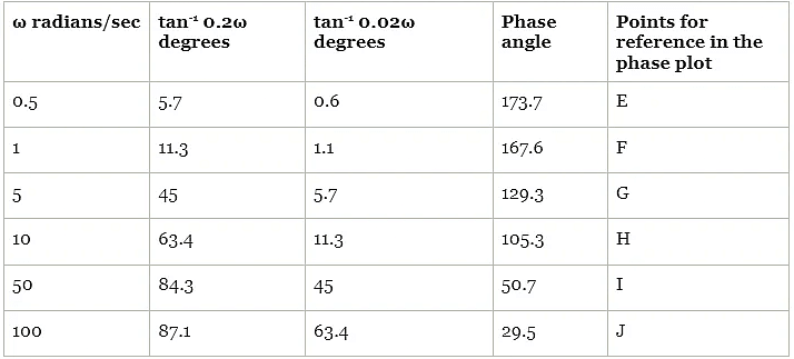
We can consider the approximated value for the given values of the phase angle.

Step 5: Calculation of the value K
The value of gain K at frequency 5 radians per second is 28 db. Hence, at every point of magnitude plot is obtained by shifting the plot wit K = -1 by -28db downwards.
Thus, the term -28db is contributed by the term K.
20 log K = -28db
Log K = -28/20 = 0.0398
The magnitude plot and the phase plot are shown below: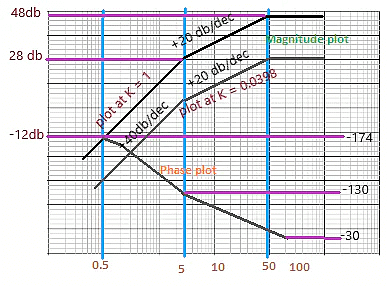

Exact value of the plot

We know that the exact plot is 3 db less than the actual plot. Thus, for the exact plot, the term -28 db+ 3db = -25db is contributed by the term K.
20 log K = -25db
Log K = -25/20 = 0.0562

Advantages of the Bode Plot

• It covers low frequency as well as high frequency.
• The Bode plot provides the relative stability of the system in terms of the gain margin and phase margin.
• It can be drawn both for the closed loop system and open-loop system.
• It also provides us a method to improve the stability of the system.
• It converts the multiplication of magnitudes into addition.
• The sketching of bode plots is derived from a simple method.
• The information loss is very less.
• It consists of two graphs that eliminate the confusion between the magnitude and the phase plots.
• Bode plot is based on the asymptotic approximations that use straight line segments for plotting on the semilog graph.

Disadvantages of the Bode Plot

• The fundamental behavior of the system does not change frequently. Hence, the bode plot is not sensitive to the changes occurring in the measuring system.
• It does clearly predict the individual contribution of different factors in the given transfer functions.