Types of Controllers | Control Systems - Electrical Engineering (EE) PDF Download

Introduction

• A controller is basically a unit present in a control system that generates control signals to reduce the deviation of the actual value from the desired value to almost zero or lowest possible value. It is responsible for the control action of the system so as to get accurate output.
• The method of producing a control signal by the controller is known as control action.
• The figure below represents the block diagram of an industrial controller:
  
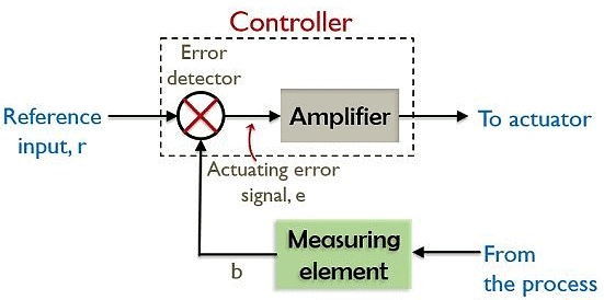
• Basically the deviation of the achieved output from the reference input is the error signal which is needed to be compensated by the controller so that the system generates required output.
• So, in a control system, the controller provides the desired controlling to the system so as to get the necessary output. Here in this article, we will discuss the various types of controllers.

Types of Controllers

• Before discussing the various types of controllers, one must be aware of the operational modes of the controllers. This is so because the various types of controllers are originated from the different modes of operation.
• So, basically there are two modes of operation:
  

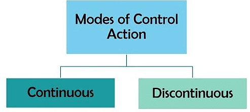
1. Discontinuous
A discontinuous mode of controller operation permits a discrete output value. In this mode, the output does not show smooth variation according to the signal generated by the controller rather shows fluctuation from one value to another.
According to this mode of operation, controllers are of two types:

• On-Off / Two-position controllers
• Multiposition controllers

2. Continuous
This mode permits smooth variation of the controlled output over the entire range of operation. The output of the control system shows continuous variation in proportion to the entire error signal or some form of it.
So, on the basis of the input applied, controllers are majorly classified as:

• Proportional controller
• Integral controller
• Derivative controller

Two-position controllers

• These are also known as on/off controllers. Here the output of the controller fluctuates between two specific values, generally the maximum and minimum value.
• The maximum value is generally considered 100% while the minimum as 0%.
• It is the easiest and most common type of control action of a controller. Here the output shows variation between maximum and minimum values according to the actuating error signal.
• Basically the output gets changed from minimum value to maximum value when the value of actuating error signal increases above a critical value.
• Similarly, the output gets reduced to its minimum value from the maximum value when the value of the error signal falls below the critical value.
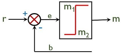
• Suppose m is the output of the controller, e represents the actuating error signal and m₁ and m₂ represent the maximum and minimum value respectively.
• Then mathematically we can write it as:
  m = m₁ (100) when e > 0
  m = m₂ (0) when e > 0
• The figure below represents the block diagram of the two-position controller:
  
• It is noteworthy in case of on-off controllers that each time when error increases or decreases through 0 then an overlapping exists. This overlapping leads to the span of error and this span of error is known as the dead zone.
• Examples of systems using two-position controllers are room heater system, liquid level controlling system in water tanks, air conditioners, etc.

Proportional Controller

• In this type of controller, a proportional linear relationship is maintained between the controlled variable and the actuating error signal.
• Suppose m is the output of the controller and e represents the error signal then for proportional controller it can be written as
  m (t) = K_Pe (t)
• Here K_P is the proportional gain constant and it determines the relation between controlled output and error signal.
• In terms of Laplace transform the above equation can be written as:
  M(S) = K_PE(s)
• Thus
  Kp = M(s)/E(s)
• So, we can say each error value provides a unique controller output in this case.
• As we have discussed that there exists a linear relationship between controller output and the error signal. But the output of the controller must not be 0 because 0 value of the error signal will give rise to halt state in the process.
• Thus for zero error, the output will be:
  m(t) = K_P E(t) + m₀
  : m_o is controlled output in case of zero error.
• This type of controller permits both direct as well as reverse action. This is so because an error can be either positive or negative depending upon the difference of reference input and the feedback signal.
• When with the increase in the input to the controller its output also increases then it is known as direct control action.
• While if the increase in input causes a decrease in output and vice-versa then it is known as reverse action.

Integral Controller

• A controller with a type of control action, in which the rate of change of the output shows proportionality with the actuating error signal is known as an integral controller.
• It can be mathematically written as
  
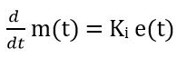
  : Ki represents the constant
• Thus the above equation can be written as
  m(t) = Ki ∫ e(t) + m(0)
  : m(0) is the output of the controller at t = 0
• In the case of the integrating controller, the rate of change of the output of the controller depends on the integrating time constant, till the time error signal becomes 0. Thus it is said to be comparatively slower than the proportional controller.
• Here in order to generate an appreciable output comparatively more time is required. But in its case, the processing continues, till the time error signal becomes zero.

Derivative Controller

• In the derivative type of controller, the controller output depends on the rate with which the error signal varies.
• Practically we can say that the error is a function of time and at any given time instant it can be 0. However, it is not necessary that it will remain zero even after that instant of time.
• Thus there must be some action that specifies the rate of change of error signal. Sometimes it is also referred as a rate action mode of the controller.
• Thus it is given as:
  
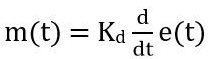
  : Kd denotes the derivative gain constant which shows the amount of variation in output of the controller for every per second rate of change of actuating error signal.
• For the above equation, Laplace transform is given as
  M(S) = Kd S.E(s)
• Or we can write it as
  M(s)/E(s) S K_d
• Hence we can say that every rate of change of error signal provides a significantly different value of the output of the controller.
• It serves as an advantageous factor for the system because every time the output varies with the change in error signal, thereby providing significant corrected output before the error approaches a large value.
• Practically these modes are not used separately thus a combination of these modes is used.

So, the combinations are as follows:

• Proportional Integral Controller: This type of controller is formed by the merger of proportional and integral control action.
  The mathematical expression for this type of controller is given as: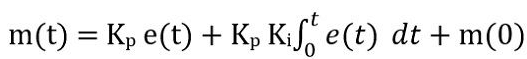
  
  : m(0) represents the initial output at t = 0.
• Proportional Derivative Controller: When proportional control action is serially combined with derivative control action then it is known as the proportional derivative controller.
  Mathematically it is expressed as: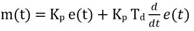
  
• Proportional Integral Derivative Controller: The control action combining all the three modes i.e., proportional, integral and the derivative is known as proportional, integral and derivative controller or PID controller.
  Mathematically it is given as: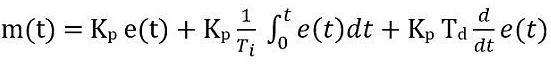
  
  So, this is all about the controller and its types.