Nyquist Plot | Control Systems - Electrical Engineering (EE) PDF Download

Introduction
- The extension of the polar plot is known as the Nyquist plot. The frequency in the case of the Nyquist plot varies from -infinity to infinity. The primary difference between the polar plots and the Nyquist plot is that the polar plots are based on frequencies range from zero to infinity, while the Nyquist plot also deals with negative frequencies.
- The Nyquist criteria help us determine the closed-loop system's stability from the frequency response of the open-loop poles and plot.
- We know that F(s) is a function of s. The polynomial in the numerator and denominator of the system in terms of s can be represented as:
F(s) = (s - z1)(s - z2)... (s - zm)/(s - p1)(s - p2)... (s - pn) - The roots of the numerator, when equated to zero, determine the zeroes of the system, and the root of the denominator determines the poles of the system. It means that the given function has m number of zeroes and n number of poles. The numerical value of n is usually greater or equal to m.
- S in the function is a complex variable, and it is given by σ + jω. Thus, F(s) is also a complex function that can be represented in the form u + jv.
- It means that for every point of s in the s-plane at which the F(s) is analytic, there exists a corresponding point in the F(s) plane. The function f(s) maps into the f(s) plane. There is a contour that maps on the contour on the other side.
- In the Nyquist plot, we will detect the presence of the closed-loop system poles in the right half of the s-plane to determine the system's stability. It is because the Nyquist plot relates the open loop frequency response (given by G(jω)H(jω)) to the number of poles and zeroes of 1 + G(s)H(s) that lie in the right-half of the s-plane.
Contour in s-Plane
- The direction of the contour in the s-plane can either enclose or encircle the point in the s-plane, and the point can be a zero or a pole. First, let's discuss the concept of encircle and enclose because both terms are useful while implementing the Nyquist stability criterion.
- Encircled: If a point is said to lie inside the closed path, it is said to be encircled. It is shown below:
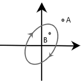 Here, point B is encircled in the closed path in a clockwise direction, while the point A lies outside the path.
 - Enclosed: If a point lies to the right side of path when the path is traversed in a specific direction, it is said to be enclosed by a closed path. Let's consider two closed path in the clockwise and anticlockwise direction, as shown below:

- The shaded region represents the region enclosed by the closed path. In the first figure, point B lies to the right when traversed in the clockwise direction, while A does not. Thus, point B is said to be enclosed by a closed path. Similarly, point A lies to the right when traversed in the anticlockwise direction in the second figure, while B does not. Thus, point A is said to be enclosed by a closed path.
Nyquist Stability Criteria
- The closed loop transfer function is given by:
C(s)/R(s) = G(s)/(1 + G(s)H(s))
Where,
C(s) is the output of the given control system
R(s) in the input of the given control system
H(s) is the feedback path
G(s) is the forward path of a system - The characteristic equation of the system is given by the condition 1 + G(s)H(s) = 0.
- We know that G(s)H(s) in terms of zeroes and poles is given by:

- The value of m is less or equal to n. It means that for an ideal control system, the number of zeroes is always less than or equal to the number of poles in a given control system.
Let, F(s) = 1 + G(s)H(s) - Putting the value of G(s)H(s) in the above equation, we get:

- Thus, z1', z2'... zn' are the zeroes of the function F(s).
- Now, let's combine the values of G(s), 1 + G(s)H(s) in the transfer function, which is given by:
C(s)/R(s) = G(s)/(1 + G(s)H(s))

- z1', z2', z3', and zn' are the poles of the above transfer function.
- The Nyquist stability criterion is based on the point -1 + j0 to determine the stability of the closed loop system. It is because the contour of the function F(s) with respect to the origin of the plane is same as the contour of the F(s) -1 plane with respect to the point -1 + j0.
- The point -1 + j0 on the axis will appear as:

Let's discuss the Nyquist stability criteria in terms of encirclement, anticlockwise encircle, and clockwise encirclement.
- Encirclement of point -1 + j0
There should be no encirclement of point -1 + j0. We know that the system is stable if the poles are present on the left half of the s-plane. Here, no encirclement means that the system is stable if there are no poles on the right side of the s-plane. The poles present on the right half of the s-plane makes the system unstable. - Anticlockwise encirclements of point -1 + j0
The anticlockwise encirclements of the point -1 + j0 are equal to the number of poles present in the right half of the s-plane. If such encirclements are not equal to the number of poles, the system becomes unstable.
For example,
A given system has two poles. For the system to be stable, the encirclements of the point -1 + j0 should also be two. - Clockwise encirclements of point -1 + j0
There should be no clockwise encirclements of the point -1 + j0 in the Nyquist plot to stabilize the system. If such encirclements are present in the plot, the system is always unstable.
Stability Analysis to draw the Nyquist Plot
The steps that will help in the stability analysis to draw the Nyquist plot.
1. Determining the poles and zeroes
- From the given transfer function, we need to determine the poles and zeroes to check the valid points.
2. Selecting a Nyquist plot
- We need to select a Nyquist plot that should enclose all the poles and zeroes present on the right-half of the s-plane except the singular points. The singular points are considered as the points lying on the imaginary axis. Hence, these points are avoided.
- If the transfer function has a pole at zero or origin, the contour encloses all the poles and zeroes except the origin.
- If there are no poles on the imaginary axis, the contour will appear as:

- Both the avoided points (origin and imaginary) in the contour are shown below:

- For mapping, the contour needs to be analytical. Let's first discuss about mapping.
3. Mapping a contour
- A singular point (point on the imaginary axis) is not analytical. Hence, it is generally avoided. The Nyquist contour is mapped to determine the encirclement of the point -1 + j0. The contour is drawn based on the transfer function is G(s)H(s).
- There are four sections C1, C2, C3, and C4. The Nyquist criterion pot is divided into four sections so that the process can be easily carried out section wise. At last, all the sections are combined to produce the desired Nyquist plot. Let the four sections be:
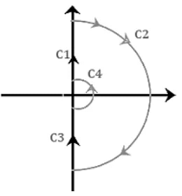 The order of these sections is somewhat similar as shown above.
4. Range for the first section C1
- We know that the Nyquist range is from -infinity to infinity, and the value of ω in section C1 ranges from 0 to infinity. The contour will be drawn in G(s)H(s) plane with respect to the above range, and it will be the locus plot of G(jω)H(jω).
- We can use various methods of mapping the first section C1, such as sketching the locus from the given transfer function, finding the frequency by equating the real and imaginary parts to zero, using the polar plot method (type and order of the system), and separating the magnitude and the phase..
5. Range for the second section C2
- The second section is generally of infinite radius. Here, it is a semi-circle of infinite radius. The range of the second section is from -90 degrees to +90 degrees. It can be obtained by:

- If the transfer function is in the form G(s)H(s) = K(1 + sT)/s(1 + sT1)(1 + sT2), the term (1 + sT) can be assumed as sT.
- The value of the transfer function at the specific value of theta will be:

Where,
N is the number of poles and m is the number of zeroes. The value of n is greater than or equal to m.
6. Range for the second section C3
- In the third section C3, the value of ω ranges from -infinity to zero. The locus of the third section is just the inverse of the polar plot of G(jω)H(jω). We can also say that it is the inverse of the first section. The resulted plot will be the mirror image of the polar with respect to the real axis.
7. Range for the second section C4
- The argument of the forth section varies from-90 degrees to 90 degrees. The Nyquist contour of this section has a semicircle of zero radii. The mapping of the section C4 is given by the condition:

- If the transfer function is in the form G(s)H(s) = K(1 + sT)/sy(1 + sT1)(1 + sT2), the term (1 + sT) can be assumed as 1.
- The value of the transfer function at the specific value of theta will be:

Where,
Y is the number of poles.
Note: If there are no poles at the origin of the Nyquist plot, the section C4 will be absent.
Example: Draw the Nyquist plot for the system whose open loop transfer function is given by:
G(s)H(s) = K/s(s + 2)(s + 10)
Also determine the range of K for which the system is stable.
The transfer function is given by:
G(s)H(s) = K/s(s + 2)(s + 10)
Step 1: Determining the poles and zeroes.
Since, the transfer function has no numerator in terms of s, there are no zeroes present in the function. There are only three poles.
G(s)H(s) = K/sx20(s/2 + 1)(s/10 + 1)
G(s)H(s) = 0.05K/s(1 + 0.5s)(1 + 0.1s)
The open loop function has a pole at the origin, which is shown below:
Now, we will perform the mapping of all four sections separately. At last, all four sections will be combined to produce the desired results.
Step 2: Mapping of section C1
The value of ω in section C1 ranges from 0 to infinity. The contour will be drawn in G(s)H(s) plane with respect to the above range will be the locus plot of G(jω)H(jω).
G(s)H(s) = 0.05K/s(1 + 0.5s)(1 + 0.1s)
G(jω)H(jω) = 0.05K/ jω(1 + 0.5jω)(1 + 0.1jω)
G(jω)H(jω) = 0.05K/ jω(1 + 0.6jω - 0.05ω2)
G(jω)H(jω) = 0.05K/-0.6 ω2 + jω(1 - 0.05ω2)
The corresponding imaginary term will be 0 and the resulted frequency will be the crossover phase frequency, which is given by:
ω(1 - 0.05ω2) = 0
1 - 0.05ω2 = 0
ω = 4.472 radians/second = crossover phase frequency
Now, we will put the value of the above frequency in the real part of the G(jω)H(jω), which is given by:
G(jω)H(jω) = 0.05K/-0.6 ω2
G(jω)H(jω) = 0.05K/-0.6x 4.472 x 4.472
G(jω)H(jω) = -0.00417K
From the given transfer function, we can easily determine that the system is of type 1 and order 3.
The polar plot will start at -90 degrees, crosses the point -0.00417K on the real axis, as shown below:
Step 3: Mapping of section C2
The range of the second section is from -90 degrees to +90 degrees. It can be obtained by:
If the transfer function is in the form G(s)H(s) = 0.05K/s(1 + 0.5s)(1 + 0.1s), the term (1 + sT) can be assumed as sT. It is given by:
G(s)H(s) = 0.05K/s x 0.5s x 0.1s
G(s)H(s) = 0.05K/0.05s3
G(s)H(s) = K/s3
Let, the value of s be:

The value of the transfer function at the specific value of theta will be:
Thus, the section C2 varying from -270 degrees to 270 degrees will appear as the plane shown in the below image:

Step 4: Mapping of section C3
We know that the section C3 is simply the inverse of section C1. Thus, the locus plot of the section C3 will be the increase on the real axis at the same point, as shown below:
Step 5: Mapping of section C4
Let's plot the C4 section of the Nyquist plot.
Let's plot the C4 section of the Nyquist plot.
The argument of the fourth section varies from-90 degrees to 90 degrees. The Nyquist contour of this section has a semicircle of zero radii. The condition gives the mapping of the section C4:
If the transfer function is in the form G(s)H(s) = 0.05K/s(1 + 0.5s)(1 + 0.1s), the term (1 + sT) can be assumed as 1. It is given by:
G(s)H(s) = 0.05K/s x 1 x 1
G(s)H(s) = 0.05K/s
Let, the value of s be:
The value of the transfer function at the specific value of theta will be:

We can say that the section C4 is mapped in the s-plane as a circular arc of infinite radius. The locus is shown below:
Step 6: Stability analysis
We will find the value of K when the contour passes through the point (-1 + j0).
-0.00417K = -1
The limiting value of K will be:
K = 1/0.00417
K = 240
Step 7: Complete Nyquist plot
The complete Nyquist plot after combining all the above four sections are shown below:

We will find the stability at the two values of K.
K< 240
- When the value of K is less than 240, the contour does not cross the real axis, and the point -1 + j0 is not encircled. There are no poles on the right half of the s-plane. Hence, the system at this value of K is stable.
K>240
- When the value of K is greater than 240, the contour crosses the real axis, and the point -1 + j0 is encircled two times in the clockwise direction. There are no poles on the right half of the s-plane. Hence, the system at this value of K is unstable.
Thus, for the stability of the given transfer function, the value of K is 0 < K < 240.
Advantages of the Nyquist Plot
- It can determine the stability of the control system.
- It is better than the root locus in terms of time delay. It means that the Nyquist plot can easily handle the time delay in the system.
- It provides a way to use the bode plots.
- It can find the frequency response of the open-loop transfer function.
- It can find the number of poles present on the right side of the s-plane.
- It can also find the relative stability of the system.
Disadvantages of the Nyquist Plot
- It uses some complex mathematical techniques.
- It cannot determine the absolute stability of the system.
- It does not provide the exact information of the number of poles present on the right side of the s-plane.
|
53 videos|107 docs|40 tests
|
FAQs on Nyquist Plot - Control Systems - Electrical Engineering (EE)
| 1. What is a Nyquist plot and what are its advantages? |  |
| 2. What are the disadvantages of using a Nyquist plot? | |
| 3. How can Nyquist plots be used to analyze stability? | |
| 4. Can Nyquist plots be used for nonlinear systems? | |
| 5. How can Nyquist plots be used for control system design? | |


MCQs
,Important questions
,video lectures
,ppt
,Previous Year Questions with Solutions
,Summary
,past year papers
,practice quizzes
,Nyquist Plot | Control Systems - Electrical Engineering (EE)
,Objective type Questions
,Viva Questions
,Nyquist Plot | Control Systems - Electrical Engineering (EE)
,Extra Questions
,mock tests for examination
,Nyquist Plot | Control Systems - Electrical Engineering (EE)
,shortcuts and tricks
,study material
,Semester Notes
,Sample Paper
,Exam
,Free
;


Nyquist Plot Free PDF Download
Importance of Nyquist Plot
Nyquist Plot Notes
Nyquist Plot Electrical Engineering (EE) Questions
Study Nyquist Plot on the App
|
© EduRev
|
Education Revolution
|


|


