Matrix Diagonalization | Engineering Mathematics - Engineering Mathematics PDF Download

Introduction
Let A and B be two matrices of order n. B can be considered similar to A if there exists an invertible matrix P such that B=P^{-1} A P This is known as Matrix Similarity Transformation.
Diagonalization of a matrix is defined as the process of reducing any matrix A into its diagonal form D. As per the similarity transformation, if the matrix A is related to D, then
D = P-1 AP and the matrix A is reduced to the diagonal matrix D through another matrix P. Where P is a modal matrix)
Modal matrix: It is a (n x n) matrix that consists of eigen-vectors. It is generally used in the process of diagonalization and similarity transformation.
In simpler words, it is the process of taking a square matrix and converting it into a special type of matrix called a diagonal matrix.
Steps Involved:
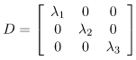
Step 1: Initialize the diagonal matrix D as: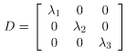
where λ1, λ2, λ3 -> eigen values
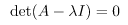
Step 2: Find the eigen values using the equation given below.
det(A-λI)=0
where, A -> given 3×3 square matrix. I -> identity matrix of size 3×3. λ -> eigen value.
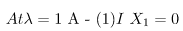
Step 3: Compute the corresponding eigen vectors using the equation given below.
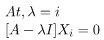
where, λi -> eigen value. Xi -> corresponding eigen vector.
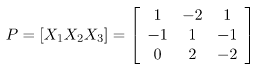
Step 4: Create the modal matrix P.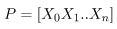
Here, all the eigenvectors till Xi have filled column-wise in matrix P.
Step 5: Find P-1 and then use the equation given below to find diagonal matrix D.
D=P-1 AP
Example Problem
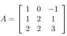
Problem Statement: Assume a 3×3 square matrix A having the following values:
Find the diagonal matrix D of A using the diagonalization of the matrix. [ D = P-1AP ]
Step 1: Initializing D as:
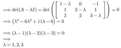
Step 2: Find the eigen values. (or possible values of λ)
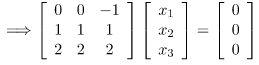
Step 3: Find the eigen vectors X1, X2, X3 corresponding to the eigen values λ = 1,2,3.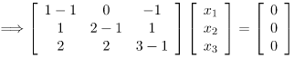
On solving, we get the following equation
x3 = 0 (x1)x1 + x2 = 0
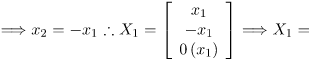
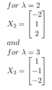
Similarly, for λ = 2
and for
similarly
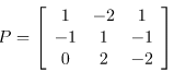
Step 5: Creation of modal matrix P. (here, X1, X2, X3 are column vectors)
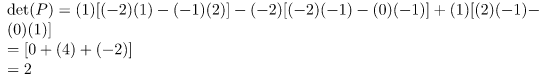
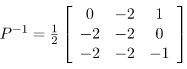
Step 6: Finding P-1 and then putting values in diagonalization of a matrix equation. [D = P-1AP]
We do Step 6 to find out which eigenvalue will replace λ1, λ2, and λ3 in the initial diagonal matrix created in Step 1.
Since det(P) ≠ 0 ⇒ Matrix P is invertible
we know that
On solving, we get
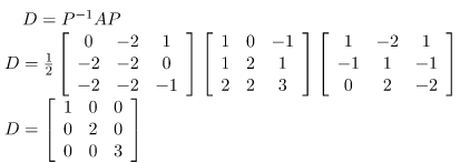
Putting in the Diagonalization of Matrix equation, we get


|
65 videos|129 docs|94 tests
|
FAQs on Matrix Diagonalization - Engineering Mathematics - Engineering Mathematics
| 1. What is matrix diagonalization? |  |
| 2. How is matrix diagonalization useful? | |
| 3. Can every matrix be diagonalized? | |
| 4. How do you diagonalize a matrix? | |
| 5. Can a matrix have multiple diagonalizations? | |


Summary
,Sample Paper
,practice quizzes
,shortcuts and tricks
,mock tests for examination
,video lectures
,study material
,Objective type Questions
,Matrix Diagonalization | Engineering Mathematics - Engineering Mathematics
,Viva Questions
,Matrix Diagonalization | Engineering Mathematics - Engineering Mathematics
,past year papers
,Semester Notes
,MCQs
,Previous Year Questions with Solutions
,Matrix Diagonalization | Engineering Mathematics - Engineering Mathematics
,Important questions
,Free
,Exam
,Extra Questions
,ppt
;


Matrix Diagonalization Free PDF Download
Importance of Matrix Diagonalization
Matrix Diagonalization Notes
Matrix Diagonalization Engineering Mathematics Questions
Study Matrix Diagonalization on the App
|
© EduRev
|
Education Revolution
|


|


within 7 days!