Echelon Form | Engineering Mathematics - Engineering Mathematics PDF Download

How to Change a Matrix Into its Echelon Form
A matrix is in row echelon form (ref) when it satisfies the following conditions.
- The first non-zero element in each row, called the leading entry, is 1.
- Each leading entry is in a column to the right of the leading entry in the previous row.
- Rows with all zero elements, if any, are below rows having a non-zero element.
A matrix is in reduced row echelon form (rref) when it satisfies the following conditions.
- The matrix is in row echelon form (i.e., it satisfies the three conditions listed above).
- The leading entry in each row is the only non-zero entry in its column.
A matrix in echelon form is called an echelon matrix. Matrix A and matrix B are examples of echelon matrices.
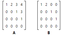 Matrix A is in row echelon form, and matrix B is in reduced row echelon form.
How to Transform a Matrix Into Its Echelon Forms
Any matrix can be transformed into its echelon forms, using a series of elementary row operations. Here's how.
- Pivot the matrix
- Find the pivot, the first non-zero entry in the first column of the matrix.
- Interchange rows, moving the pivot row to the first row.
- Multiply each element in the pivot row by the inverse of the pivot, so the pivot equals 1.
- Add multiples of the pivot row to each of the lower rows, so every element in the pivot column of the lower rows equals 0.
- To get the matrix in row echelon form, repeat the pivot
- Repeat the procedure from Step 1 above, ignoring previous pivot rows.
- Continue until there are no more pivots to be processed.
- To get the matrix in reduced row echelon form, process non-zero entries above each pivot.
- Identify the last row having a pivot equal to 1, and let this be the pivot row.
- Add multiples of the pivot row to each of the upper rows, until every element above the pivot equals 0.
- Moving up the matrix, repeat this process for each row.
Transforming a Matrix Into Its Echelon Forms: An Example
To illustrate the transformation process, let's transform Matrix A to a row echelon form and to a reduced row echelon form.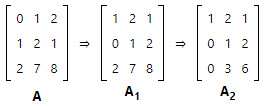
 To transform matrix A into its echelon forms, we implemented the following series of elementary row operations.
- We found the first non-zero entry in the first column of the matrix in row 2; so we interchanged Rows 1 and 2, resulting in matrix A1.
- Working with matrix A1, we multiplied each element of Row 1 by -2 and added the result to Row 3. This produced A2.
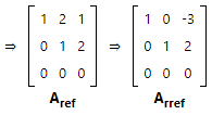
- Working with matrix A2, we multiplied each element of Row 2 by -3 and added the result to Row 3. This produced Aref. Notice that Aref is in row echelon form, because it meets the following requirements: (a) the first non-zero entry of each row is 1, (b) the first non-zero entry is to the right of the first non-zero entry in the previous row, and (c) rows made up entirely of zeros are at the bottom of the matrix.
- And finally, working with matrix Aref, we multiplied the second row by -2 and added it to the first row. This produced Arref. Notice that Arref is in reduced row echelon form, because it satisfies the requirements for row echelon form plus each leading non-zero entry is the only non-zero entry in its column.
Note: The row echelon matrix that results from a series of elementary row operations is not necessarily unique. A different set of row operations could result in a different row echelon matrix. However, the reduced row echelon matrix is unique; each matrix has only one reduced row echelon matrix.
|
65 videos|129 docs|94 tests
|
FAQs on Echelon Form - Engineering Mathematics - Engineering Mathematics
| 1. What is echelon form in linear algebra? |  |
| 2. How is echelon form different from reduced echelon form? | |
| 3. What are the benefits of using echelon form in linear algebra? | |
| 4. How can a matrix be transformed into echelon form? | |
| 5. Can every matrix be transformed into echelon form? | |


practice quizzes
,Echelon Form | Engineering Mathematics - Engineering Mathematics
,Important questions
,Exam
,study material
,mock tests for examination
,Previous Year Questions with Solutions
,ppt
,Free
,Viva Questions
,Semester Notes
,past year papers
,Sample Paper
,Echelon Form | Engineering Mathematics - Engineering Mathematics
,Echelon Form | Engineering Mathematics - Engineering Mathematics
,shortcuts and tricks
,Summary
,video lectures
,Objective type Questions
,MCQs
,Extra Questions
;


Echelon Form Free PDF Download
Importance of Echelon Form
Echelon Form Notes
Echelon Form Engineering Mathematics Questions
Study Echelon Form on the App
|
© EduRev
|
Education Revolution
|


|


within 7 days!