State Space Model

The state space model of Linear Time-Invariant (LTI) system can be represented as,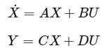
The first and the second equations are known as state equation and output equation respectively. Where,
- X and X˙ are the state vector and the differential state vector respectively.
- U and Y are input vector and output vector respectively.
- A is the system matrix.
- B and C are the input and the output matrices.
- D is the feed-forward matrix.
Basic Concepts of State Space Model
The following basic terminology involved in this chapter.
State
It is a group of variables, which summarizes the history of the system in order to predict the future values (outputs).
State Variable
The number of the state variables required is equal to the number of the storage elements present in the system.
Examples - current flowing through inductor, voltage across capacitor
State Vector
It is a vector, which contains the state variables as elements.
In the earlier chapters, we have discussed two mathematical models of the control systems. Those are the differential equation model and the transfer function model. The state space model can be obtained from any one of these two mathematical models. Let us now discuss these two methods one by one.
State Space Model from Differential Equation
Consider the following series of the RLC circuit. It is having an input voltage, vi(t) and the current flowing through the circuit is i(t) .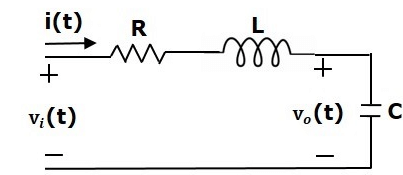
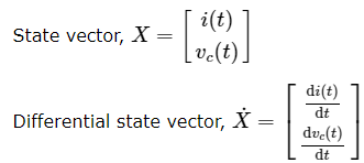
There are two storage elements (inductor and capacitor) in this circuit. So, the number of the state variables is equal to two and these state variables are the current flowing through the inductor, i(t) and the voltage across capacitor, vc(t) . From the circuit, the output voltage, v0(t) is equal to the voltage across capacitor, vc(t) .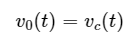 Apply KVL around the loop.
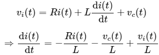
The voltage across the capacitor is -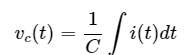 Differentiate the above equation with respect to time.
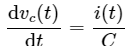
We can arrange the differential equations and output equation into the standard form of state space model as,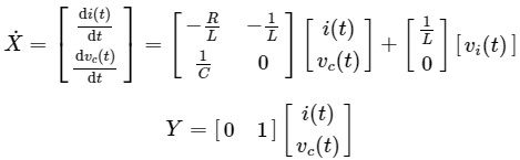 Where,
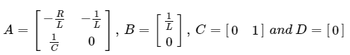
State Space Model from Transfer Function
Consider the two types of transfer functions based on the type of terms present in the numerator.
- Transfer function having constant term in Numerator.
- Transfer function having polynomial function of 's' in Numerator.
Transfer function having constant term in Numerator
Consider the following transfer function of a system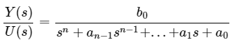 Rearrange, the above equation as
 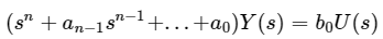 Apply inverse Laplace transform on both sides.
 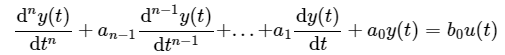 Let
Let 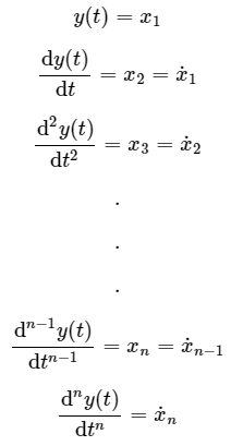 and u(t)=u
Then,  From the above equation, we can write the following state equation.
 The output equation is -
 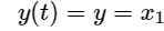 The state space model is -
 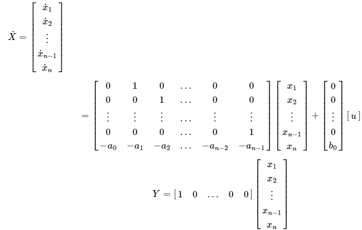 Here, D=[0].
Example: Find the state space model for the system having transfer function.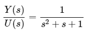 Rearrange, the above equation as,
Apply inverse Laplace transform on both the sides. 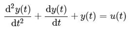 Let
Let 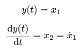
and u(t)=u
Then, the state equation is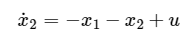 The output equation is
 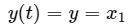 The state space model is
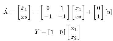
Transfer function having polynomial function of 's' in Numerator
Consider the following transfer function of a system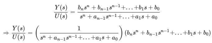 The above equation is in the form of product of transfer functions of two blocks, which are cascaded.
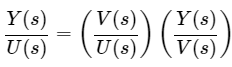 Here,
Here, 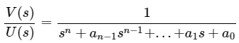 Rearrange, the above equation as
 Apply inverse Laplace transform on both the sides.
 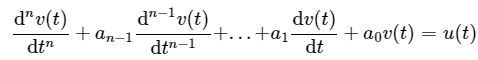 Let
Let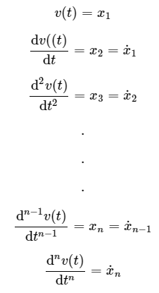
and u(t)=u
Then, the state equation is Consider
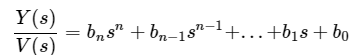 Rearrange, the above equation as
 Apply inverse Laplace transform on both the sides.
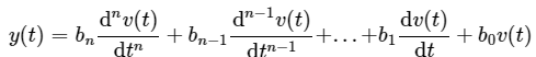 By substituting the state variables and y(t)=y in the above equation, will get the output equation as,
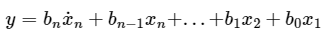 Substitute, x˙n value in the above equation.
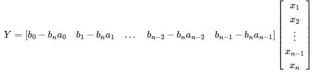
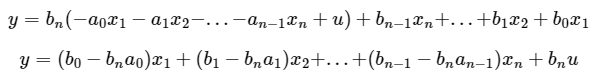 The state space model is
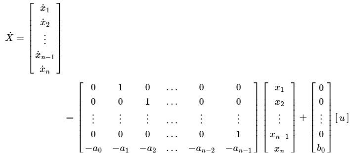
 If bn=0 , then,
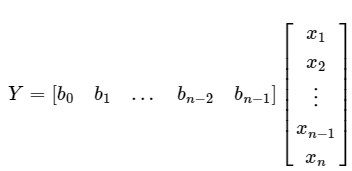
FAQs on State Space Model
| 1. What are the basic concepts of a State Space Model? |  |
| 2. How can a State Space Model be derived from a set of differential equations? | |
| 3. How can a State Space Model be obtained from a transfer function? | |
| 4. What does it mean when a transfer function has a constant term in the numerator? | |
| 5. What is the significance of having a polynomial function of 's' in the numerator of a transfer function? | |


|
Explore Courses for Electrical Engineering (EE) exam
|
|

|
Get EduRev Notes directly in your Google search
|
|