Modelling of Physical Systems | Control Systems - Electrical Engineering (EE) PDF Download
| Table of contents |

|
| Modelling Electrical Systems |

|
| Series RLC Network |

|
| Parallel RLC Network |

|
| Mechanical Systems |

|
| The Analogy |

|
Although physical systems include a wide variety of systems, we shall restrict ourselves to electrical and mechanical systems in this tutorial. A mathematical model is the mathematical representation of the physical system which is made using the appropriate governing laws of that system. These governing laws are Ohm’s law and Kirchhoff's laws for electrical systems and when it comes to mechanical systems, we use Newton’s laws of motion. These laws help us in obtaining the relation between the input and output of the system.
For most physical systems, a mathematical model is a set of differential equations. A system is said to be linear if its mathematical model obeys the principle of superposition and homogeneity. This means that if a system outputs y1 and y2 to x1 and x2 respectively, then the system output to the linear combination of these inputs a1x1 + a2x2 should be the linear combination of their individual outputs a1y1 + a2y2 for the system to be linear. Here a1 and a2 are constants.
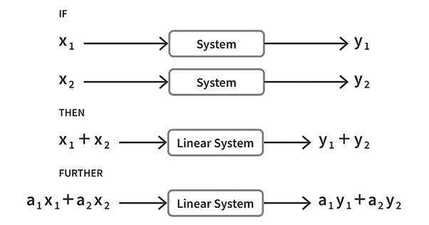
Although most systems are non linear, they are made linear through certain assumptions in order to apply techniques developed for linear systems that we shall discuss in the upcoming tutorials. This helps make the analysis of system behaviour easier. In this entire tutorial series we shall be restricting ourselves to the analysis of linear time invariant (LTI) systems i.e., systems that are linear and the variables in the differential equations are independent of time. The mathematical models of LTI systems can be reshaped into a transfer function which we shall learn about in the next tutorial.
We shall now discuss electrical and mechanical systems individually and show how to develop their mathematical models.
Modelling Electrical Systems
Electrical circuits have three basic elements, the resistor, the capacitor and the inductor. These are analyzed based on Kirchhoff’s laws as stated before. The voltage-current relationships of these elements are as shown below in both time domain and in laplace domain.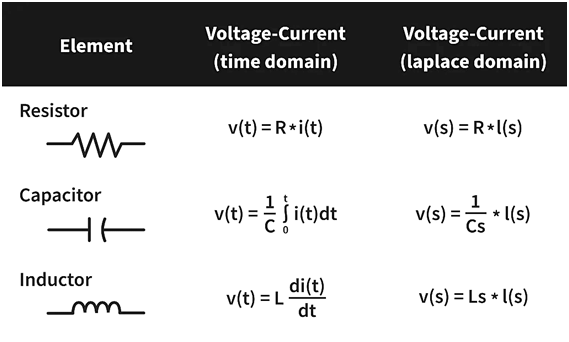 With this, now we can proceed to develop mathematical models for a series RLC network and then for a parallel RLC network.
Series RLC Network
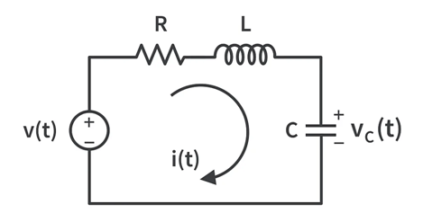
A mathematical model usually defines the relation between an input and an output. Hence, first we must decide the input and the output. In this network let’s choose vc(t) as the output and v(t) as input as it’s the only one in this network.
Then, to find the relationship between the input and output, we start by applying Kirchhoff’s voltage law around the loop, assuming the initial conditions to be zero, obtaining,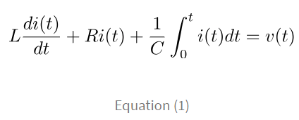 But the goal is to find the relationship between the input and output *voltages* - which the left hand side of the equation is in terms of current. But the current is the rate of flow of charges and by replacing i(t) by dq(t)/dt in the above equation, we get:
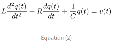
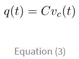 So we can substitute q(t) in equation (2) using equation (3), we obtain,
This equation is the mathematical model for the series RLC network. Notice that on the left hand of the equation, everything is in terms of the voltage across the capacitor, vc(t), with the input of v(t). We successfully created a mathematical equation that relates the input and the output. With this equation, we should be able to calculate what will happen in a real circuit given an input and component parameters. And, later, we’ll learn about how to convert this to the Laplace domain and how it’ll help us. But for now, let’s be content with what we’ve accomplished thus far.
Parallel RLC Network
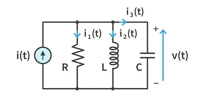 In this network, i(t) is the input and output is taken as v(t).
Applying Kirchhoff’s current law for the above network, assuming initial conditions to be zero,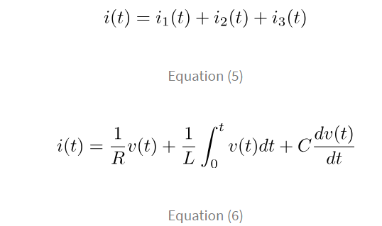
The above equation represents the mathematical model of the parallel RLC network.
For now, let’s move aside and recall Faraday’s law. It tells that the induced voltage is equal to the rate of change of the magnetic flux linking the coil, which in case is referring to the magnetic flux in the inductor (L) . Read more about Faraday’s law here:
If the magnetic flux linking the inductor is φ(t), then the voltage across the inductor can be written as v(t) = dφ/dt. Hence the modified mathematical model in terms of this flux linkage becomes,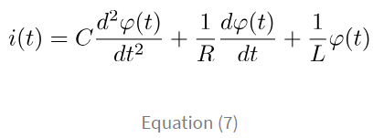 Any electrical network can be mathematically modelled in a similar manner using Kirchhoff's laws and other basic relations. Truly, the only difference between your typical circuit analysis and mathematical modeling of electric circuits is explicitly creating equations and relationships between an input and output, rather than solving for particular values.
Mechanical Systems
Mechanical systems are usually classified into translational systems and rotational systems. These are modelled by three translatory and three rotatory elements as shown below.
Translational Systems
In translational motion, the motion is along a straight line. There are three types of elements that oppose this motion.
1) The mass element or the inertia element.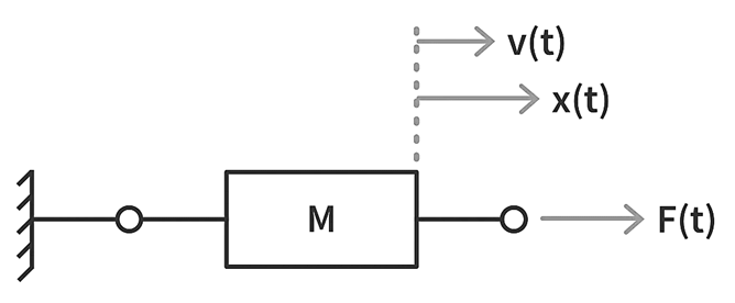 The mass element represents the system’s inertia. As per Newton’s second law of motion, the inertia force shall be equal to the rate of change of linear momentum and hence,
 where,
M = Mass
F(t) = Force
v(t) = velocity
x(t) = displacement
In other words, force is equal to mass times the change in velocity, or mass times acceleration.
2) The spring element.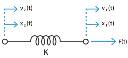 The spring element represents the potential energy storage elements in the mechanical systems. The restoring force of a spring is directly proportional to the net displacement [ x1(t) - x2(t) ] of the spring.
 where,
K = spring constant or the stiffness
In other words, the force the spring exerts is equal to the stiffness of the spring multiplied by the amount the spring is stretched.
3) The damper element. The damper element is responsible for the viscous friction in the system. The damping torque is directly proportional to the net angular velocity of the element.
 where,
B = Damping coefficient
Now, let’s model a simple translational and a rotational system.
Translational System
Consider the below translational system with the usual notations as discussed earlier.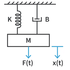 Here, F(t) is the force that is serving as the input to the system and we consider the displacement x(t) as the output. When we equate this applied force to the sum of all the opposing forces on the system, we obtain
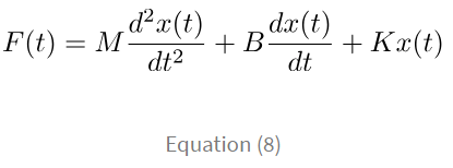 The above equation represents the mathematical model of the given translational system. It’s easier than the circuit models we went over earlier simply because we didn’t need to change the units we were working in.
Rotational System
Consider the below rotational system with the usual notations as discussed earlier. We consider a shaft which is connected to a wheel of moment of inertia J at one end and rigidly mounted on the other side. External torque T(t) is applied on the wheel which causes an angular displacement θ(t) and B represents the coefficient of friction betweens the wheel and the ground.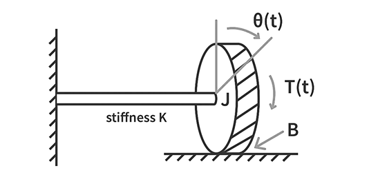 Here, T(t) is the external torque that serves as the input to the system and we consider the angular displacement θ(t) as the output.
When we equate this applied torque to the sum of all the opposing torques on the system, we obtain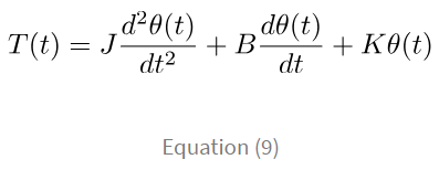
The above equation represents the mathematical model of the given rotational system. In a similar manner, all mechanical systems can be modelled.
The Analogy
Until now, we have understood how we can model electrical and mechanical systems. Now let’s take a look at some interesting relations. Let’s now compare the mathematical models of a series RLC network (equation (2)) and the discussed translational system [equation (8)] and rotational system [equation (9)].
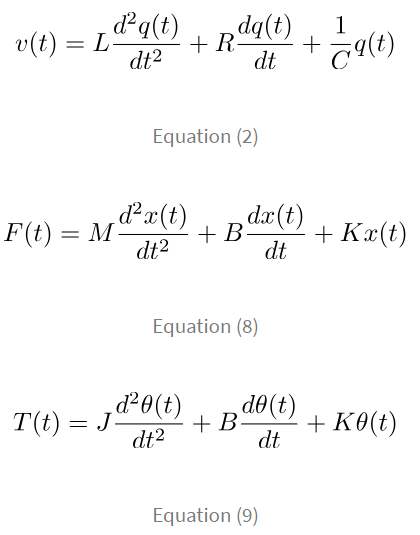
Do you find any similarities in these three equations? That’s right, they have the same structure. Here, the force F(t) and torque T(t) are analogous to the voltage v(t) and hence, this analogy is called the force-voltage analogy. Now let’s tabulate the other analogous quantities in this analogy.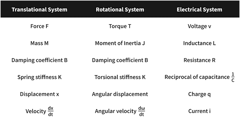
Now again, let’s now compare the mathematical models of a parallel RLC network [equation (7)] and the discussed translational system [equation (8)] and rotational system [equation (9)].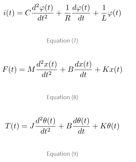 Do you see any similarities? Again, it’s the same structure but here the force F and torque T are analogous to the current i. Hence this type of analogy is called the force-current analogy. In a similar fashion, we shall tabulate the other analogous quantities in this analogy.
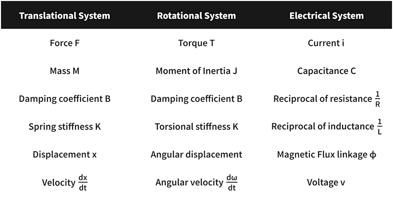 We can convert a mechanical system into an electrical network by the above analogies and apply network analysis techniques to analyse the mechanical system.
|
53 videos|115 docs|40 tests
|
FAQs on Modelling of Physical Systems - Control Systems - Electrical Engineering (EE)
| 1. What are some common applications of modelling electrical systems? |  |
| 2. How does a series RLC network differ from a parallel RLC network? |  |
| 3. What is the significance of the analogy between electrical and mechanical systems in modelling physical systems? |  |
| 4. How can modelling help in optimizing the performance of electrical systems? |  |
| 5. What are some key parameters that need to be considered when modelling mechanical systems? |  |


