


All Exams >
Class 6 >
How to become an Expert of MS Excel >
All Questions
All questions of Data Analysis for Class 6 Exam
Which of the following statements about sorting data in Excel is TRUE?- a)Sorting data in Excel permanently rearranges the original data
- b)Sorting data in Excel does not affect the original data
- c)Sorting data in Excel creates a backup copy of the original data
- d)Sorting data in Excel is not possible without using VBA code
Correct answer is option 'A'. Can you explain this answer?
Which of the following statements about sorting data in Excel is TRUE?
a)
Sorting data in Excel permanently rearranges the original data
b)
Sorting data in Excel does not affect the original data
c)
Sorting data in Excel creates a backup copy of the original data
d)
Sorting data in Excel is not possible without using VBA code

|
Anshu Nishad answered |
A

Which Excel tool would you use to find the optimal solution for a complex mathematical problem involving multiple variables and constraints?- a)One Variable Data Table
- b)Two Variable Data Table
- c)Goal Seek
- d)Solver
Correct answer is option 'D'. Can you explain this answer?
Which Excel tool would you use to find the optimal solution for a complex mathematical problem involving multiple variables and constraints?
a)
One Variable Data Table
b)
Two Variable Data Table
c)
Goal Seek
d)
Solver
|
|
Rounak Chawla answered |
Introduction:
Excel is a powerful tool that offers various functionalities to help solve complex mathematical problems. When dealing with a problem involving multiple variables and constraints, the most suitable tool in Excel is the Solver.
Solver:
The Solver tool in Excel is an optimization tool that can be used to find the optimal solution for complex mathematical problems. It allows you to define the objective function, set constraints, and specify the variables' limitations. The Solver then iteratively adjusts the variables to find the optimal solution that satisfies the defined constraints and maximizes or minimizes the objective function.
How to use Solver:
To use Solver in Excel, follow these steps:
1. Set up the problem:
- Define the objective function, which is the equation to be maximized or minimized.
- Specify the variables and their limitations, such as upper and lower bounds.
- Set the constraints, which are the limitations or conditions that the solution must satisfy.
2. Open Solver:
- Click on the "Data" tab in the Excel ribbon.
- In the "Analysis" group, click on "Solver."
3. Define the Solver parameters:
- Set the objective function by selecting the cell containing the function.
- Specify the variables by selecting the cells containing the variable values.
- Set the constraints by adding them one by one.
4. Configure the Solver options:
- Choose the optimization method, such as Simplex LP or GRG Nonlinear.
- Set the target, whether it is to maximize or minimize the objective function.
- Define the tolerance for the solution.
5. Solve the problem:
- Click on the "Solve" button to start the Solver process.
- Solver will adjust the variables iteratively to find the optimal solution.
- Once Solver finds a solution, it will display the optimal values for the variables and the objective function.
Conclusion:
When dealing with a complex mathematical problem involving multiple variables and constraints in Excel, the Solver tool is the most appropriate choice. It allows you to define the objective function, set constraints, and specify the limitations on variables. By iteratively adjusting the variables, Solver finds the optimal solution that satisfies the constraints and maximizes or minimizes the objective function.
What is the significance of conditional formatting in Excel?- a)It allows you to create formulas to perform calculations.
- b)It highlights cells based on specific criteria.
- c)It enables you to create charts and graphs.
- d)It helps you to create macros for automation.
Correct answer is option 'B'. Can you explain this answer?
What is the significance of conditional formatting in Excel?
a)
It allows you to create formulas to perform calculations.
b)
It highlights cells based on specific criteria.
c)
It enables you to create charts and graphs.
d)
It helps you to create macros for automation.
|
|
Shilpa Choudhury answered |
Conditional formatting allows you to format cells based on specific conditions or criteria, making it easier to identify patterns or highlight important data.
Consider the following VBA code in Excel:
Sub ExampleCode()
Dim rng As Range
Set rng = Range("A1:A5")
MsgBox rng.Cells.Count
End Sub- a)1
- b)5
- c)6
- d)It will cause an error
Correct answer is option 'B'. Can you explain this answer?
Consider the following VBA code in Excel:
Sub ExampleCode()
Dim rng As Range
Set rng = Range("A1:A5")
MsgBox rng.Cells.Count
End Sub
Sub ExampleCode()
Dim rng As Range
Set rng = Range("A1:A5")
MsgBox rng.Cells.Count
End Sub
a)
1
b)
5
c)
6
d)
It will cause an error
|
|
Muskaan Chavan answered |
"A1:B10") For Each cell In rng If cell.Value > 10 Then cell.Interior.Color = RGB(255, 0, 0) End If Next cellEnd SubThis code defines a range of cells (A1 to B10) and then loops through each cell in that range. If the value of the cell is greater than 10, it changes the interior color of the cell to red.
This code can be used to highlight cells that meet a certain condition, such as values above a certain threshold.
This code can be used to highlight cells that meet a certain condition, such as values above a certain threshold.
What is the output of the following Excel formula: =COUNTIF(A1:A10, ">50")?- a)The number of cells in the range A1 to A10 that contain a value greater than 50.
- b)The number of cells in the range A1 to A10 that contain a value less than or equal to 50.
- c)The sum of all the values in the range A1 to A10 that are greater than 50.
- d)The average of all the values in the range A1 to A10 that are greater than 50.
Correct answer is option 'A'. Can you explain this answer?
What is the output of the following Excel formula: =COUNTIF(A1:A10, ">50")?
a)
The number of cells in the range A1 to A10 that contain a value greater than 50.
b)
The number of cells in the range A1 to A10 that contain a value less than or equal to 50.
c)
The sum of all the values in the range A1 to A10 that are greater than 50.
d)
The average of all the values in the range A1 to A10 that are greater than 50.
|
|
Priyanka Sharma answered |
The COUNTIF function counts the number of cells in a range that meet a specific criterion.
Which of the following is NOT a type of conditional formatting in Excel?- a)Color Scales
- b)Icon Sets
- c)Data Bars
- d)Pivot Tables
Correct answer is option 'D'. Can you explain this answer?
Which of the following is NOT a type of conditional formatting in Excel?
a)
Color Scales
b)
Icon Sets
c)
Data Bars
d)
Pivot Tables
|
|
Amar Singh answered |
Explanation:
Conditional formatting is a feature in Excel that allows users to apply specific formatting to cells or ranges based on certain conditions or criteria. It provides visual cues to highlight and analyze data more effectively.
The given options are:
a) Color Scales: Color scales apply different colors to cells based on their values. This helps to identify high and low values or patterns within a range of data.
b) Icon Sets: Icon sets display icons in cells based on the values they contain. Different icons represent different conditions, such as arrows indicating trends or symbols representing specific criteria.
c) Data Bars: Data bars add horizontal bars to cells proportional to their values. They provide a visual representation of the relative sizes or magnitudes of the data.
d) Pivot Tables: Pivot tables are not a type of conditional formatting. They are a powerful tool used to summarize, analyze, and present large amounts of data. Pivot tables allow users to group and arrange data, calculate totals or averages, and generate reports.
Conclusion:
Out of the given options, the correct answer is d) Pivot Tables. Pivot tables are not a type of conditional formatting; they are a separate feature in Excel used for data analysis and reporting. The other options (a, b, and c) are all valid types of conditional formatting that help users visualize and interpret data more effectively.

What does the VLOOKUP function do in Excel?- a)It performs vertical alignment of data.
- b)It allows you to view multiple sheets simultaneously.
- c)It searches for a value in the leftmost column of a table and returns a value in the same row.
- d)It provides a visual representation of data.
Correct answer is option 'C'. Can you explain this answer?
What does the VLOOKUP function do in Excel?
a)
It performs vertical alignment of data.
b)
It allows you to view multiple sheets simultaneously.
c)
It searches for a value in the leftmost column of a table and returns a value in the same row.
d)
It provides a visual representation of data.
|
|
Shilpa Choudhury answered |
The VLOOKUP function is used to search for a value in the leftmost column of a table and return a value in the same row from a specified column.
What is the output of the following Excel formula: =SUM(A1:A5)?- a)The sum of all the values in cells A1 to A5.
- b)The product of all the values in cells A1 to A5.
- c)The average of all the values in cells A1 to A5.
- d)The maximum value among all the values in cells A1 to A5.
Correct answer is option 'A'. Can you explain this answer?
What is the output of the following Excel formula: =SUM(A1:A5)?
a)
The sum of all the values in cells A1 to A5.
b)
The product of all the values in cells A1 to A5.
c)
The average of all the values in cells A1 to A5.
d)
The maximum value among all the values in cells A1 to A5.
|
|
Ashwini Goyal answered |
The correct answer is option 'A': The sum of all the values in cells A1 to A5.
Explanation:
To understand the output of the formula =SUM(A1:A5), let's break down the formula and its components.
- The formula starts with the SUM function, which is used to add up a range of cells.
- The range of cells specified in this formula is A1 to A5. This means that it will include all the values in cells A1, A2, A3, A4, and A5.
- The SUM function will add up all the values in the specified range and return the total sum.
So, the output of this formula will be the sum of all the values in cells A1 to A5.
For example, if the values in cells A1 to A5 are 5, 10, 15, 20, and 25, the formula =SUM(A1:A5) will calculate the sum as 5 + 10 + 15 + 20 + 25 = 75.
Therefore, the correct answer is option 'A': The sum of all the values in cells A1 to A5.
Which of the following is NOT a data validation option in Excel?- a)Whole number
- b)Decimal number
- c)Text length
- d)Percentage
Correct answer is option 'D'. Can you explain this answer?
Which of the following is NOT a data validation option in Excel?
a)
Whole number
b)
Decimal number
c)
Text length
d)
Percentage
|
|
Shilpa Choudhury answered |
Data validation in Excel does have an option to validate percentages, so this is not an invalid option.
What does the COUNTIF function in Excel do?- a)Counts the number of cells in a range that meet a specific criterion
- b)Calculates the average of a range of cells
- c)Adds up the values in a range of cells
- d)Checks if a cell contains a specific value
Correct answer is option 'A'. Can you explain this answer?
What does the COUNTIF function in Excel do?
a)
Counts the number of cells in a range that meet a specific criterion
b)
Calculates the average of a range of cells
c)
Adds up the values in a range of cells
d)
Checks if a cell contains a specific value
|
|
Sagar Gupta answered |
Explanation of the COUNTIF function in Excel:
Function:
The COUNTIF function in Excel is used to count the number of cells within a specified range that meet a specific criterion.
Usage:
- Syntax: COUNTIF(range, criteria)
- It takes two arguments: the range of cells you want to evaluate and the criteria that cells must meet to be counted.
Example:
- Suppose you have a range of cells (A1:A10) containing numbers and you want to count how many cells have a value greater than 5.
- You can use the COUNTIF function like this: =COUNTIF(A1:A10, ">5")
- This formula will return the count of cells in the range A1:A10 that are greater than 5.
Functionality:
- The COUNTIF function evaluates each cell in the specified range against the given criteria.
- If a cell meets the criteria, it is counted; otherwise, it is ignored.
- The function then returns the total count of cells that satisfy the condition.
Conclusion:
In summary, the COUNTIF function in Excel is a powerful tool for quickly counting cells that meet specific criteria within a range. It is commonly used in data analysis and reporting to obtain valuable insights from Excel data.
Which of the following functions is used to calculate the average of a range of cells in Excel?- a)SUM
- b)AVERAGE
- c)COUNT
- d)MAX
Correct answer is option 'B'. Can you explain this answer?
Which of the following functions is used to calculate the average of a range of cells in Excel?
a)
SUM
b)
AVERAGE
c)
COUNT
d)
MAX
|
|
Shilpa Choudhury answered |
The AVERAGE function is used to calculate the average of a range of cells in Excel.
What is the purpose of sorting data in Excel?- a)To arrange data in alphabetical order
- b)To arrange data in chronological order
- c)To organize data for easier analysis
- d)To calculate the total number of data points
Correct answer is option 'C'. Can you explain this answer?
What is the purpose of sorting data in Excel?
a)
To arrange data in alphabetical order
b)
To arrange data in chronological order
c)
To organize data for easier analysis
d)
To calculate the total number of data points
|
|
Palak Nair answered |
Purpose of Sorting Data in Excel
Sorting data in Excel serves multiple purposes, but the primary aim is to organize data for easier analysis. Here’s a detailed breakdown of why this is essential:
1. Enhanced Data Organization
- Sorting helps to systematically arrange data, making it easier to locate specific information.
- When data is organized, users can quickly find patterns and trends that may not be visible in a random arrangement.
2. Improved Analysis
- By sorting data, you can analyze subsets of information more effectively.
- For example, sorting sales data by date can help track performance over time, while sorting by customer names can highlight client behaviors.
3. Facilitates Comparisons
- Sorting allows users to compare similar data points more easily.
- When data is in order, it’s simpler to assess high and low values, making it easier to draw conclusions.
4. Informed Decision-Making
- With organized data, users can make more informed decisions based on clear insights derived from the sorted information.
- For instance, a sorted list of expenses can help identify areas to cut costs.
5. Custom Sorting Options
- Excel provides various sorting options, allowing users to sort by multiple criteria.
- This flexibility aids in deeper analysis and tailored data presentation.
In conclusion, while sorting in alphabetical or chronological order are specific applications, the broader purpose of sorting in Excel is indeed to organize data for easier analysis, enhancing clarity and insight for users.
What is the purpose of using conditional formatting with data bars in Excel?- a)To compare values within a range of cells
- b)To apply a specific color scale to cells
- c)To highlight specific cells with icons
- d)To create a histogram of cell values
Correct answer is option 'A'. Can you explain this answer?
What is the purpose of using conditional formatting with data bars in Excel?
a)
To compare values within a range of cells
b)
To apply a specific color scale to cells
c)
To highlight specific cells with icons
d)
To create a histogram of cell values
|
|
Jay Goyal answered |
Introduction:
Conditional formatting is a feature in Excel that allows users to apply formatting to cells based on specific criteria or conditions. One of the options for conditional formatting is the use of data bars, which are visual representations of the values in a range of cells. The purpose of using conditional formatting with data bars in Excel is to compare values within a range of cells.
Explanation:
Conditional formatting with data bars helps users visually analyze and compare the values in a range of cells. Here's how it works:
1. Visual Comparison:
Data bars provide a visual representation of the values in a range of cells, making it easier to compare them at a glance. The length of the data bar corresponds to the value in each cell, allowing users to quickly identify the relative magnitude of different values.
2. Relative Value Comparison:
By using data bars, users can easily determine the highest and lowest values within a range. The longer the data bar, the higher the value, and the shorter the data bar, the lower the value. This allows users to identify trends, patterns, and outliers in the data.
3. Proportional Comparison:
Data bars also enable users to compare the values in different cells proportionally. The length of the data bar represents the proportion of each value relative to the maximum value in the range. This helps users understand the distribution of values and identify cells with significantly higher or lower values.
4. Customization:
Excel provides various customization options for data bars, allowing users to modify their appearance according to their preferences. Users can choose different colors, adjust the width of the data bars, and even display the values within the bars to provide additional context.
5. Conditional Formatting:
Conditional formatting with data bars can be applied to a range of cells based on specific conditions. For example, users can set a rule that applies data bars to highlight cells with values above a certain threshold or within a certain range. This allows for further customization and focus on specific data points.
Conclusion:
The purpose of using conditional formatting with data bars in Excel is to compare values within a range of cells. Data bars provide a visual representation that facilitates the analysis of data, allowing users to quickly identify trends, patterns, and outliers. By customizing the appearance and applying conditional formatting, users can further enhance their ability to interpret and understand the data.
Which of the following is not a valid data type in Excel?- a)Text
- b)Number
- c)Date
- d)Image
Correct answer is option 'D'. Can you explain this answer?
Which of the following is not a valid data type in Excel?
a)
Text
b)
Number
c)
Date
d)
Image
|
|
Shilpa Choudhury answered |
Excel does not support the data type of an image. It mainly deals with text, numbers, and dates.
Which of the following sorting options in Excel arranges data in ascending order?- a)A to Z
- b)Z to A
- c)Largest to Smallest
- d)Smallest to Largest
Correct answer is option 'A'. Can you explain this answer?
Which of the following sorting options in Excel arranges data in ascending order?
a)
A to Z
b)
Z to A
c)
Largest to Smallest
d)
Smallest to Largest
|
|
Priyanka Sharma answered |
The "A to Z" sorting option in Excel arranges data in ascending order based on the selected column.
What does conditional formatting in Excel allow you to do?- a)Apply specific formats to cells based on their values
- b)Calculate complex formulas based on cell references
- c)Sort and filter data based on specific criteria
- d)Define named ranges for easier data analysis
Correct answer is option 'A'. Can you explain this answer?
What does conditional formatting in Excel allow you to do?
a)
Apply specific formats to cells based on their values
b)
Calculate complex formulas based on cell references
c)
Sort and filter data based on specific criteria
d)
Define named ranges for easier data analysis
|
|
Priyanka Sharma answered |
Conditional formatting in Excel allows you to apply different formats, such as colors, to cells based on specific conditions or rules.
Which Excel tool allows you to vary one input value to reach a desired result in another cell?- a)One Variable Data Table
- b)Two Variable Data Table
- c)Goal Seek
- d)Solver
Correct answer is option 'C'. Can you explain this answer?
Which Excel tool allows you to vary one input value to reach a desired result in another cell?
a)
One Variable Data Table
b)
Two Variable Data Table
c)
Goal Seek
d)
Solver
|
|
Anita Menon answered |
Goal Seek allows you to vary one input value to find the desired result in another cell.
Which Excel tool would you use to analyze the impact of changing interest rates on the monthly mortgage payment?- a)One Variable Data Table
- b)Two Variable Data Table
- c)Goal Seek
- d)Scenario Manager
Correct answer is option 'C'. Can you explain this answer?
Which Excel tool would you use to analyze the impact of changing interest rates on the monthly mortgage payment?
a)
One Variable Data Table
b)
Two Variable Data Table
c)
Goal Seek
d)
Scenario Manager
|
|
Anita Menon answered |
Goal Seek in Excel is used to determine the value of an input cell that will achieve a desired result in a dependent cell.
What is the output of the following Excel formula: =AVERAGEIFS(A1:A10, B1:B10, "Red")?- a)The average of all the values in the range A1 to A10 that have a corresponding value "Red" in the range B1 to B10.
- b)The sum of all the values in the range A1 to A10 that have a corresponding value "Red" in the range B1 to B10.
- c)The count of all the values in the range A1 to A10 that have a corresponding value "Red" in the range B1 to B10.
- d)The maximum value among all the values in the range A1 to A10 that have a corresponding value "Red" in the range B1 to B10.
Correct answer is option 'A'. Can you explain this answer?
What is the output of the following Excel formula: =AVERAGEIFS(A1:A10, B1:B10, "Red")?
a)
The average of all the values in the range A1 to A10 that have a corresponding value "Red" in the range B1 to B10.
b)
The sum of all the values in the range A1 to A10 that have a corresponding value "Red" in the range B1 to B10.
c)
The count of all the values in the range A1 to A10 that have a corresponding value "Red" in the range B1 to B10.
d)
The maximum value among all the values in the range A1 to A10 that have a corresponding value "Red" in the range B1 to B10.
|
|
Priyanka Sharma answered |
The AVERAGEIFS function calculates the average of values in a range that meet multiple criteria.
How can you filter data in Excel based on multiple criteria?- a)By using the "Find and Replace" dialog box
- b)By applying a specific format to the cells
- c)By using the "Filter" option in the "Data" tab
- d)By selecting cells and pressing Ctrl+F
Correct answer is option 'C'. Can you explain this answer?
How can you filter data in Excel based on multiple criteria?
a)
By using the "Find and Replace" dialog box
b)
By applying a specific format to the cells
c)
By using the "Filter" option in the "Data" tab
d)
By selecting cells and pressing Ctrl+F
|
|
Priyanka Sharma answered |
Excel provides a "Filter" option in the "Data" tab that allows you to filter data based on multiple criteria. You can select specific values, ranges, or conditions for filtering.
Consider the following data in an Excel worksheet:
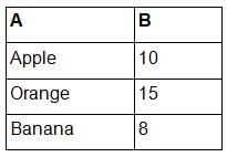
You want to highlight the fruit names (column A) that have a quantity (column B) greater than or equal to 10 using conditional formatting. Which formula can you use in the conditional formatting rule?- a)=A1>=10
- b)=$B1>=10
- c)=$B1<10
- d)=$B1>>=10
Correct answer is option 'B'. Can you explain this answer?
Consider the following data in an Excel worksheet:
You want to highlight the fruit names (column A) that have a quantity (column B) greater than or equal to 10 using conditional formatting. Which formula can you use in the conditional formatting rule?
You want to highlight the fruit names (column A) that have a quantity (column B) greater than or equal to 10 using conditional formatting. Which formula can you use in the conditional formatting rule?
a)
=A1>=10
b)
=$B1>=10
c)
=$B1<10
d)
=$B1>>=10
|
|
Shilpa Choudhury answered |
In the conditional formatting rule, you should use the formula =$B1>=10 to highlight the fruit names (column A) where the corresponding quantity (column B) is greater than or equal to 10.
What is the purpose of data validation in Excel?- a)To ensure that formulas in a worksheet are correct
- b)To check for errors in the data entered into cells
- c)To perform mathematical calculations on data in a worksheet
- d)To filter and sort data in a worksheet
Correct answer is option 'B'. Can you explain this answer?
What is the purpose of data validation in Excel?
a)
To ensure that formulas in a worksheet are correct
b)
To check for errors in the data entered into cells
c)
To perform mathematical calculations on data in a worksheet
d)
To filter and sort data in a worksheet
|
|
Shilpa Choudhury answered |
Data validation in Excel helps ensure that the data entered into cells meets specific criteria or conditions. It can be used to prevent errors or inconsistencies in the data.
How can you create a named range in Excel?- a)Using the "Name Manager" dialog box
- b)Applying a specific format to a range of cells
- c)Assigning a specific value to a range of cells
- d)Writing a specific formula in a range of cells
Correct answer is option 'A'. Can you explain this answer?
How can you create a named range in Excel?
a)
Using the "Name Manager" dialog box
b)
Applying a specific format to a range of cells
c)
Assigning a specific value to a range of cells
d)
Writing a specific formula in a range of cells
|
|
Shilpa Choudhury answered |
The "Name Manager" dialog box in Excel allows you to create, edit, and delete named ranges. You can access it from the "Formulas" tab.
Which of the following best describes a named range in Excel?- a)A range of cells with a specific name assigned to it
- b)A range of cells with a specific format assigned to it
- c)A range of cells with a specific value assigned to it
- d)A range of cells with a specific formula assigned to it
Correct answer is option 'A'. Can you explain this answer?
Which of the following best describes a named range in Excel?
a)
A range of cells with a specific name assigned to it
b)
A range of cells with a specific format assigned to it
c)
A range of cells with a specific value assigned to it
d)
A range of cells with a specific formula assigned to it
|
|
Shilpa Choudhury answered |
A named range in Excel is a range of cells that has been given a specific name. This name can be used in formulas and functions to refer to the range instead of using cell references.
Which Excel tool is used to create and manage multiple sets of input values for a scenario analysis?- a)One Variable Data Table
- b)Two Variable Data Table
- c)Goal Seek
- d)Scenario Manager
Correct answer is option 'D'. Can you explain this answer?
Which Excel tool is used to create and manage multiple sets of input values for a scenario analysis?
a)
One Variable Data Table
b)
Two Variable Data Table
c)
Goal Seek
d)
Scenario Manager
|
|
Anita Menon answered |
Scenario Manager in Excel helps create and manage multiple sets of input values for a scenario analysis.
Which of the following is a valid criterion for filtering data in Excel?- a)Text that starts with a specific letter
- b)Cells that contain a formula
- c)Values greater than a specific cell reference
- d)All of the above
Correct answer is option 'D'. Can you explain this answer?
Which of the following is a valid criterion for filtering data in Excel?
a)
Text that starts with a specific letter
b)
Cells that contain a formula
c)
Values greater than a specific cell reference
d)
All of the above
|
|
Priyanka Sharma answered |
All the mentioned criteria are valid options for filtering data in Excel.
What is the purpose of filtering data in Excel?- a)To remove duplicates from a range of cells
- b)To rearrange data based on specific criteria
- c)To apply specific formats to cells
- d)To calculate mathematical formulas
Correct answer is option 'B'. Can you explain this answer?
What is the purpose of filtering data in Excel?
a)
To remove duplicates from a range of cells
b)
To rearrange data based on specific criteria
c)
To apply specific formats to cells
d)
To calculate mathematical formulas
|
|
Priyanka Sharma answered |
Filtering data in Excel allows you to display only the data that meets specific criteria or conditions, making it easier to analyze or work with a subset of the data.
What is the output of the following Excel formula: =IF(A1>B1, "Yes", "No")?- a)"Yes" if the value in cell A1 is greater than the value in cell B1; otherwise, "No".
- b)"No" if the value in cell A1 is greater than the value in cell B1; otherwise, "Yes".
- c)"Yes" if the value in cell A1 is equal to the value in cell B1; otherwise, "No".
- d)"No" if the value in cell A1 is equal to the value in cell B1; otherwise, "Yes".
Correct answer is option 'A'. Can you explain this answer?
What is the output of the following Excel formula: =IF(A1>B1, "Yes", "No")?
a)
"Yes" if the value in cell A1 is greater than the value in cell B1; otherwise, "No".
b)
"No" if the value in cell A1 is greater than the value in cell B1; otherwise, "Yes".
c)
"Yes" if the value in cell A1 is equal to the value in cell B1; otherwise, "No".
d)
"No" if the value in cell A1 is equal to the value in cell B1; otherwise, "Yes".
|
|
Ishaan Chawla answered |
The formula =IF(A1 has an incomplete syntax and will result in an error. The IF function requires three arguments: a logical test, the value to be returned if the test is true, and the value to be returned if the test is false.
Which of the following is NOT a valid use of named ranges in Excel?- a)Simplifying complex formulas by using named ranges instead of cell references
- b)Defining specific criteria for data validation
- c)Creating dynamic charts that automatically update with new data
- d)Grouping related cells together for easier data analysis
Correct answer is option 'B'. Can you explain this answer?
Which of the following is NOT a valid use of named ranges in Excel?
a)
Simplifying complex formulas by using named ranges instead of cell references
b)
Defining specific criteria for data validation
c)
Creating dynamic charts that automatically update with new data
d)
Grouping related cells together for easier data analysis
|
|
Sarita Singh answered |
Named ranges are not directly related to data validation. They are used to simplify formulas and cell references, create dynamic charts, and group related cells.
Chapter doubts & questions for Data Analysis - How to become an Expert of MS Excel 2025 is part of Class 6 exam preparation. The chapters have been prepared according to the Class 6 exam syllabus. The Chapter doubts & questions, notes, tests & MCQs are made for Class 6 2025 Exam. Find important definitions, questions, notes, meanings, examples, exercises, MCQs and online tests here.
Chapter doubts & questions of Data Analysis - How to become an Expert of MS Excel in English & Hindi are available as part of Class 6 exam.
Download more important topics, notes, lectures and mock test series for Class 6 Exam by signing up for free.
How to become an Expert of MS Excel
92 videos|62 docs|15 tests
|
|
© EduRev
|
Education Revolution
|


|


Signup on EduRev and stay on top of your study goals
10M+ students crushing their study goals daily