Production Function Class 12 Economics

Introduction
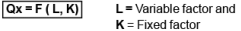
Meaning: The production function illustrates the connection between the physical inputs a firm utilizes and the physical outputs it generates. It is denoted as:
Qx = f(X1, X2, X3 ....) This signifies that the output relies on various inputs, encompassing both factors and non-factors. When focusing solely on labor and capital as inputs, the production function is represented as:
Technical Relationship : This concept represents the maximum output that can be achieved from specific inputs. For example, the function can be expressed as 50 = f(10, 2), indicating that a maximum of 50 units can be produced with 10 units of labor and 2 units of capital.
Short Run

In the short run, a firm is unable to change all inputs, leading to the presence of fixed factors that remain constant.
Long Run
The long run refers to the period when a firm can adjust all the inputs used in the production process.
| Basis | Short Run | Long Run |
|---|---|---|
| Meaning | A period where output can change by modifying only variable factors. | A period where output can change by adjusting all factors of production. |
| Classification | Involves both fixed and variable factors. | All factors are variable. |
| Price Determination | Demand plays a larger role since supply cannot be immediately increased. | Both demand and supply equally influence price determination. |
Understanding Production Period and Outputs

The production period is a concept that varies based on the conditions of production and can be different for each firm and industry. For example:
- In the steel industry, a 10-year period might be considered short due to the long-term nature of steel production.
- Conversely, for a wheat producer, a one-year period could be seen as a long-run period because of the quicker turnaround in wheat production.
Example of Production
- A farmer employs one unit of labor on his land and yields five quintals of wheat.
- This scenario illustrates the change in total production resulting from the addition of one more unit of a variable factor while keeping other factors constant.
- If the farmer is joined by his son on the same land, then 2 units of labor produce 7 quintals of wheat.
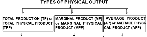
Marginal Product (MP)
- MP is calculated by finding the difference in total production before and after adding the extra unit of labor.
- In this case, MP = 7 - 5 = 2 quintals.
Average Product (AP)
- AP represents the per-unit production of the variable factor used in the production process.
- In this example, AP = Total Production / Total Labor Units = 7 quintals / 2 units = 3.5 quintals.
 It refers to change in totalproduction due to application of one more unit of variable factor other factor remaining constantEx: - If on same land father is joined by his son and thus 2 units of labour produces 7 quintal of wheat then MP = 7-5 = 2 quintals
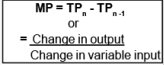
Ex: - If on same land father is joined by his son and thus 2 units of labour produces 7 quintal of wheat then MP = 7-5 = 2 quintals
It ref ers p er unit production of variable factor used in the process of productionExample :: AP of father and son is = 7/2 = 3.5 quintals
Example :: AP of father and son is = 7/2 = 3.5 quintals
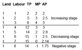
RELATION BETWEEN AP AND MP
(1) Both are derived from TP as MP = TPn - TPn -1 and AP = TP / L
(2) AP is rising MP is above it
(3) MP cuts AP when AP is at maximum point
(4) AP is falling MP is below it
(5) MP can be zero and negative but AP cannot be.

THAT MP CAN FALL WHEN AP IS RISING :: MP reaches its maximum point earlier than AP as it is faster and thereafter starts falling from point “A” to “C” where as AP is rising from “B” to “C”. Thus it can be concluded that MP can fall when AP is rising
SHAPE OF AP AND MP IS INVERSE U - SHAPE
WHY MP IS FASTER :: It must be noted that both AP and MP are derived from TP.
⇒ AP is calculated on the basis of ALL THE UNITS whereas ⇒ MP is based on ADDITIONAL UNIT ONLY. So , it is the MP THAT PULLS THE AP UP OR DOWN
WHY MP CUT AP AT ITS MAXIMUM :: It happens because when AP rises , MP is more than AP. W hen AP falls , MP is less than AP. So it is only when AP is constant and at its maximum point that MP is equal to AP. Therefore , MP cuts AP curve at its maximum point
WHY MP IS NEGATIVE :: MP is negative due to EXCESSIVE EMPLOYMENT or DISGUISED EMPLOYMENT (as in case of Agriculture sector or Public Sector Undertaking). Excessive employment which means employment of more workers than required reduces overall efficiency of the worker and makes MP negative
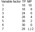
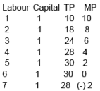
RELATIONSHIP BETWEEN MP AND TP
(1) TP = Σ MP = MP1 MP2 MP3 ................ MPn.
This means that every additional output adds to total output
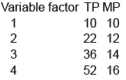
(2) TP is INCREASING AT INCREASING RATE WHEN MP IS POSITIVE AND INCREASING
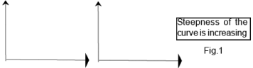
(3) TP is INCREASING AT CONSTANT RATE WHEN MP IS POSITIVE AND CONSTANT
(4) TP INCREASES AT DIMINISHING RATE MP IS POSITIVE BUT DECREASES
(5) TP is MAXIMUM WHEN MP IS ZERO (i.e MP touches X - axis)
(6) TP FALLS WHEN MP IS NEGATIVE (i.e below X - axis)
 Steepness of the curve is decreasing
RETURN TO FACTOR
MEANING :: It explain the BEHAVIOUR OF OUTPUT IN SHORT PERIOD when input of one factor is increased while all other factor remains constant. In other words it TELLS CHANGES IN OUTPUT WHEN THERE IS CHANGE IN FACTOR RATIO as more and more of variable factor is employed with same fixed factors in short period.
(1) INCR EASING RETUR N TO FACTOR :: It re fers to situ ation when given percentage INCREASE IN VARIABLE FACTOR only causes proportionate MORE increase in output
⇒ In other words MARGINAL PRODUCT of the variable factor must be INCREASING and total output tends to increase at the increasing rate
Reasons for Increasing Returns to a Factor

1. Fuller Utilization of Fixed Factors
- When the variable factor is increased while keeping the fixed factors constant (such as machinery) in the short run, it leads to better utilization of the previously underused fixed factors.
- This improved utilization enhances the efficiency of fixed factors, resulting in an increase in marginal product (MP).
- Example: In a small textile factory, if the optimal number of workers is five, hiring only one or two workers leads to inefficient production. As more workers are added, the inefficiencies decrease, leading to better utilization of the factory.
2. Increase in Efficiency
- Economists such as Adam Smith, Marshall, and Mrs. Joan Robinson argue that increasing the number of variable factors allows for greater division of labor and specialization.
- This can result in savings in training, equipment, and time, thereby applying the law of increasing returns under certain conditions.
3. Better Coordination Between Factors
- There is an improvement in the coordination between variable and fixed factors.
- This enhanced coordination boosts productivity and increases total output.
4. Indivisibility of Fixed Factor
- This concept refers to the necessity of certain fixed factors to produce goods up to a specific limit.
- Example: An economic teacher can efficiently teach up to 30 students. If the number of students drops to 15, the teacher cannot be reduced in number.
Constant Return to Factor and Diminished Return to Factor

(2) Constant Return to Factor: This concept refers to a scenario where a certain percentage increase in a variable factor leads to an identical proportionate increase in output. In simpler terms, it means that the marginal product of the variable factor remains constant, resulting in a steady increase in total output at the same rate.
Causes of Constant Returns: Optimum utilization of the fixed factor: When the fixed factor is utilized at its optimum level, it contributes to a constant increase in output with the variable factor. Ideal factor ratio: Maintaining an ideal ratio between the variable and fixed factors ensures that the marginal product remains constant, leading to consistent output growth. Most efficient utilization of the variable factor: When the variable factor is used most efficiently, it maximizes output without diminishing returns, resulting in constant returns to scale.
(3) Diminished Return to a Factor or the Law of Diminishing Returns: This principle describes a situation where a certain percentage increase in variable input leads to a smaller proportionate increase in output. In this case, the marginal product of the variable factor is decreasing, eventually reaching zero and then becoming negative with each additional unit of the variable factor.
Causes for Decreasing Return to Factor: Increased inefficiency in production: As production becomes less efficient, the marginal product of the variable factor decreases, leading to diminishing returns. Overcrowding of inputs: When too many inputs are used in production, it can lead to overcrowding, reducing the effectiveness of each input and causing diminishing returns. Decreased productivity of the variable factor: If the productivity of the variable factor declines, it results in a lower marginal product, contributing to diminishing returns.
Fixity of Factor
- Fixity of Factor refers to the overuse of fixed resources, which can lead to their breakdown. This situation results in halted production, increased costs, and decreased efficiency.
- Imperfect Factor Substitute : According to Mrs. John Robinson, labor cannot be replaced by capital indefinitely. Therefore, adding more labor to the same amount of capital will eventually result in lower returns.
- Poor Coordination : When there are too many variable factors mixed with fixed factors, it disrupts coordination and creates management challenges. This disruption can lead to a decrease in total product (TP).
- Beyond Optimum Production : Once a fixed factor is used optimally, adding more variable factors can cause diminishing returns. This occurs because the balance between fixed and variable factors becomes ineffective.
- For instance, consider a machine as a fixed factor of production. It operates best with four laborers. If a fifth laborer is added, the increase in production will be minimal because the marginal product of the additional laborer will decline.
Law of Variable Proportion (LOVP)
- Definition : The Law of Variable Proportion states that when the quantity of a variable factor changes, the Total Physical Product (TPP) initially increases at a faster rate, then at a slower rate, and eventually starts to decline.
- In simpler terms, when the variable factor is increased, the total product experiences changes at different speeds. This concept is referred to as the Law of Variable Proportion (LOVP).
Introduction
The Law of Variable Proportions (LOVP) is also referred to as the "Law of Return" or the "Law of Return to Factor." This concept is an extension of the Law of Diminishing Returns, as it considers both the phases of increasing and decreasing Marginal Product (MP).
Special Point
- LOVP is an extension of the Law of Diminishing Returns as it takes into account phases of both rising and falling Marginal Product (MP).
Assumptions
- One of the factors is variable while all other factors remain fixed.
- All units of the variable factor are homogeneous or equally efficient.
- There is no change in the technique of production.
- Factors of production can be used in different proportions. For example, 2 hectares of land with 1 labourer; or 2 hectares of land with 4 labourers.
- Operates in the short period.
- Adequate or standard doses of the variable factor are applied.
Stage I
In Stage I, the firm is moving towards the optimal mix of production factors. Total Production (TP) is increasing rapidly, indicating potential for higher profits. The firm will continue to produce by utilizing more variable factors, which will enhance profitability.
Stage II
- In Stage II, the firm experiences the advantages of increasing returns but is nearing the point of diminishing returns.
- During this stage, production decisions are guided by the Law of Diminishing Marginal Returns.
- The law states that adding more of one input while keeping others constant will eventually lead to a decrease in additional output.
Stage III
Stage III is characterized by declining profits due to:
- (a) Increased costs associated with using more variable factors
- (b) Decreased revenue resulting from reduced output
Stages I and III are both considered stages of economic absurdity.
Conditions of Applicability or Causes of Application
- Causes of Increasing Returns to Factor: Factors that contribute to increasing returns when additional inputs are added.
- Causes of Diminishing Returns to Factor: Factors that lead to diminishing returns as more inputs are added.
Postponement of the Law
- Introduction of New Technology: The Law of Diminishing Returns becomes ineffective when new technology is introduced, resulting in higher productivity and lower costs.
- Perfect Substitutability of Production Factors: The law may be postponed when production factors can perfectly substitute each other, eliminating the limitation of fixed factors.
|
1335 videos|1436 docs|834 tests
|
FAQs on Production Function Class 12 Economics
| 1. What is a production function? |  |
| 2. How is the production function calculated? | |
| 3. What are the different types of production functions? | |
| 4. What is the significance of the production function in economics? | |
| 5. How does technology affect the production function? | |


Viva Questions
,shortcuts and tricks
,Production Function Class 12 Economics
,practice quizzes
,mock tests for examination
,ppt
,Production Function Class 12 Economics
,Free
,Production Function Class 12 Economics
,Previous Year Questions with Solutions
,video lectures
,Extra Questions
,Sample Paper
,study material
,Semester Notes
,Important questions
,MCQs
,past year papers
,Exam
,Summary
,Objective type Questions
;


Chapter Notes - Production Function Free PDF Download
Importance of Chapter Notes - Production Function
Chapter Notes - Production Function
Chapter Notes - Production Function SSC CGL Questions
Study Chapter Notes - Production Function on the App
|
© EduRev
|
Education Revolution
|


|


