
Best Study Material for Commerce Exam
Commerce Exam > Commerce Notes > Economics Class 11 > Chapter Notes - The Theory of the Firm under Perfect Competition
Revenue Class 12 Economics
| Table of contents |
|
| What is a Market? |
|
| Perfect Competition: Defining Features |
|
| Revenue |
|
| Profit Maximisation |
|
| Supply Curve of a Firm |
|
| Determinants of Supply Curve |
|
| Market Supply Curve |
|
What is a Market?
A market is a mechanism or arrangement that brings buyers and sellers of a commodity or service together and allows them to complete the act of selling and buying the commodity or service at mutually agreed prices.

Perfect Competition: Defining Features
- In a perfect competition market, numerous buyers and sellers compete for the same products at the same price, with no restrictions on entering or leaving the market and no government intervention.
- All firms offer a uniform product, meaning that one firm's product is indistinguishable from another's.
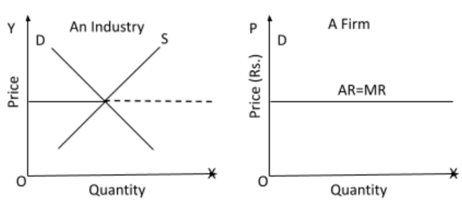
- The demand curve for each firm in this market is perfectly elastic, appearing as a horizontal line at the market price.
- Prices are set by the market, so the price a firm charges matches the market price, indicating that the firm has no control over pricing.
- No single firm can affect the market price of the product.
- Firms aim to maximise profits, which means they accept the market price set by the industry.
- All buyers and sellers have complete information about prices, quality, and other important details regarding the products and the market.
- The large number of buyers and sellers means that each buyer and seller is relatively small compared to the overall market.
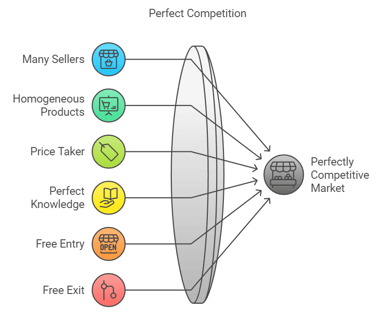
Features of Perfect Competition
- A large number of sellers: In a perfectly competitive market, there are a large number of small sellers selling homogeneous products to their buyers. The number of sellers is so large that no single firm can influence the overall market price or market supply. Hence no individual seller by altering its sale or supply can impact the overall market supply or market price.
- Homogeneous Products: Each company creates and sells a uniform product. i.e., one firm's product cannot be distinguished from the product of any other firm.
- Price Taker: In this form of market, the firm is a price taker, and not a price maker, as the share of each firm in the market is so insignificant as to impact the price of the commodity. Firms have the freedom to enter and quit the market at any time.
- Perfect knowledge about the markets: It implies that the consumers and producers have all the relevant market-related information. Producers will not be ready to sell at any price below the market price while consumers will not be ready to buy at any price above the existing market price. This eliminates the price differences in the market and helps in quickly achieving the equilibrium level of the price level.
- Free entry: Free Entry means that there are no obstacles to the entry of new firms into the market. When the existing businesses are earning abnormal profits, the new firms are influenced due to the profit and they enter the industry. This increases market supply which leads to a fall in market price and profits.
- Free exit: Freedom to exit means that there are no obstacles that stop the existing firms from stepping down from the market. The firms attempt to quit when they are dealing with losses. As the firms start to exit, market supply drops, which begins to rise in market price and consequently decreases in losses. The firms do not stop leaving till the losses are eliminated and each remaining firm will be earning just the normal profits.
- Perfect Mobility: In a perfectly competitive market, the factors of production are perfectly mobile, and hence can be easily transferred from one firm to the other.
Question for Chapter Notes - The Theory of the Firm under Perfect Competition
Try yourself:
What is a characteristic of perfect competition?View Solution
Revenue
- It is the revenue received by a company from the sale of a product or service to its clients.
Total Revenue (TR)
- The price (p) of the commodity is multiplied by the amount produced and sold to determine revenue (q).
- Total revenue (TR) is defined as
TR=p×q in algebraic form.
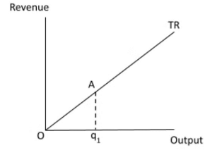
Total Revenue Curve
- The relationship between the total revenue earned by a firm for selling its output and the quantity of output sold is visually represented by a curve.
- To determine economic profit and the profit-maximizing level of production, it is paired with a firm's total cost curve.
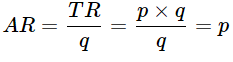
Average Revenue
- The income earned per unit of output is referred to as average revenue.
- In other words, it is the profit earned by the seller on each unit of the commodity sold.
- The average revenue of a company is calculated by dividing total revenue by total output.
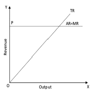
Price Line In Perfect Competition
- The price line and demand curve for an individual firm in a completely competitive market are the same.
- The line denotes that a company's goods and services may be sold at the current price.
- The price line in such a market is a horizontal straight line that depicts that the firm can sell any quantity of a product only at a certain price. If the firm tries to change the price, the overall demand falls to zero, because as there are a large number of small firms, no firm is capable enough to impact the overall price or supply.
- The price line is shown below:

Marginal Revenue
- The revenue generated by selling an additional unit of a commodity is known as marginal revenue.
- When an additional unit of a commodity is sold on the market, it results in a change in overall revenue.
- The following equations can be used to describe the link between market price and marginal revenue:
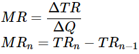
TR = Total Revenue
MR = Marginal Revenue
Q = Quantity - In a perfectly competitive market, the price equals marginal revenue, according to the preceding equation.
MR = PQn − PQn-1
or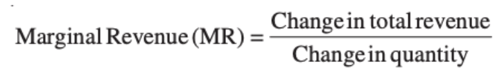
Understanding Marginal Revenue with an Example
Imagine you have a small bakery selling cupcakes.
- When you sell 2 cupcakes, you earn Rs. 30.
- When you sell 3 cupcakes, you earn Rs. 45.
Now, let’s find out how much extra money you made by selling that 1 extra cupcake.
- Change in Total Revenue = Rs. 45 - Rs. 30 = Rs. 15.
- Change in Quantity = 3 - 2 = 1.
So, Marginal Revenue (MR) = 15/1 = Rs. 15.
That means, by selling 1 more cupcake, you earned an extra Rs. 15.
Is Marginal Revenue Always the Same as Price?
Yes! For a bakery in a perfectly competitive market, the Marginal Revenue (MR) is always equal to the market price (p).
The relationship between MR and Price
We can prove that MR = Price (p) under perfect competition:
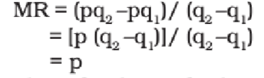
The relationship between marginal revenue and pricing is depicted graphically as follows: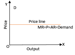
TR, MR and AR Curves in a Perfectly Competitive Market
Profit Maximisation
Imagine a toy-making company that produces and sells a certain number of toys. The company's profit (π) is simply the difference between the money it earns from selling toys (Total Revenue, TR) and the money it spends on making them (Total Cost, TC). So,
Profit (π) = TR – TC.
The bigger the gap between TR and TC, the higher the profit. Naturally, the company wants to make this gap as big as possible. But how do they find the perfect number of toys to produce (q0) to get the most profit?
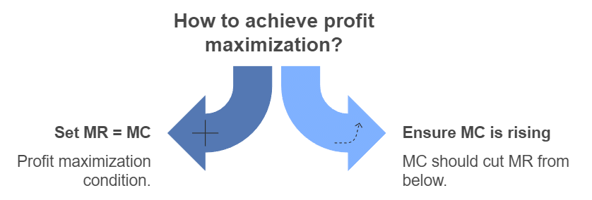
To Maximize Profit, These Conditions Must Be Met:
- Price (p) must equal Marginal Cost (MC): The company makes the most profit when the money earned from selling one more toy is exactly the same as the cost of making that toy.
- Marginal Cost Should Not Decrease at q0: The cost of making each extra toy shouldn’t keep dropping at the profit-maximizing point.
- Price Must Cover Costs:
- Short Run: The price should be higher than the Average Variable Cost (AVC).
- Long Run: The price should be higher than the Average Cost (AC).
Condition 1: Maximizing Profit by Comparing Revenue and Cost
A company's profit is the difference between the money it earns (Total Revenue) and the money it spends (Total Cost). As the company produces and sells more products, both Total Revenue and Total Cost increase.
Now, here's the key:
- If the extra revenue earned from selling one more unit (Marginal Revenue, MR) is greater than the extra cost of producing that unit (Marginal Cost or MC), then profits will keep increasing.
- But if the MR is less than the MC, the company’s profit decreases.
To make the most profit, the company needs to produce up to the point where Marginal Revenue equals Marginal Cost (MR = MC).
In a perfectly competitive market, MR = Price (P). So, the company will earn the most profit when it produces up to the point where P = MC.
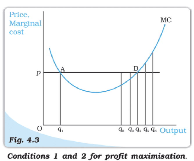
Condition 2: Why Marginal Cost Can't Slope Downward for Maximum Profit
For a firm to achieve the highest profit, the Marginal Cost (MC) curve should not be sloping downward at the profit-maximizing point. But why?
Imagine two output levels: q1 and q4. At both points, the market price is the same as the MC. However, at q1, the MC curve is sloping downward.
Now, look at the outputs slightly to the left of q1. The market price is lower than the MC. According to the profit rule we learned earlier, the company’s profit will actually be higher if it produces slightly less than q1.
Since producing at q1 doesn’t give the highest possible profit, q1 cannot be the profit-maximizing output. The MC curve must be flat or upward-sloping at the point where profit is highest.
Condition 3: Price Must Cover Costs to Keep Producing
For a firm to make the most profit, it must consider whether it’s operating in the short run or the long run.
Case 1: Short Run (Price ≥ AVC)
In the short run, a company will only keep producing if the market price is at least equal to the Average Variable Cost (AVC).
Why?
If the price is lower than the AVC, the firm is losing more money by producing than it would by simply shutting down. It’s like running a lemonade stand where each glass costs Rs. 5 to make (AVC), but you’re only able to sell them for Rs. 3. You’d be better off not selling at all!
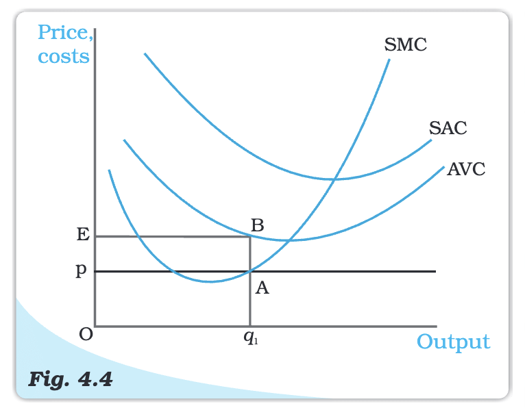
Understanding the Concept with the Figure
Imagine a firm producing at an output level q1, where the market price (p) is lower than the AVC. Here’s what happens:
- Total Revenue (TR) = Price × Quantity = Area of rectangle OpAq1.
- Total Variable Cost (TVC) = AVC × Quantity = Area of rectangle OEBq1.
Now, compare the two areas:
- The firm’s loss at q1 is: TR - TVC - TFC = (OpAq1) - (OEBq1) - TFC.
- Clearly, the revenue OpAq1 is less than the cost OEBq1.
What if the Firm Produces Nothing?
- If output = 0, then TR = 0 and TVC = 0.
- The firm’s loss would only be its Total Fixed Cost (TFC).
Since the loss at q1 is even greater than just TFC, it’s better for the firm to stop production entirely rather than produce at a loss.
In short, if the market price (p) is below the AVC, the firm will choose to produce nothing because it's losing more money by producing than by stopping.
Case 2: Price Must Cover Average Cost in the Long Run
In the long run, a profit-maximizing firm will only continue producing if the market price is equal to or above the Average Cost (AC). Let’s break down why.

Understanding the Concept with the Figure
Imagine a firm producing at an output level q1, where the market price (p) is below the Average Cost (AC). Here’s what happens:
- Total Revenue (TR) = Price × Quantity = Area of rectangle OpAq1.
- Total Cost (TC) = Average Cost × Quantity = Area of rectangle OEBq1.
Since the area representing Total Cost (OEBq1) is larger than the area representing Total Revenue (OpAq1), the firm is incurring a loss at this output level.
What if the Firm Stops Producing?
- In the long run, a firm that stops production altogether has a profit of zero.
- Producing at q1 gives a loss, so the firm would prefer to exit the market completely.
To stay in business, the market price must be at least equal to AC.
The Profit Maximization Problem: Graphical Representation
Let's understand how a firm maximizes its profit through a graphical representation.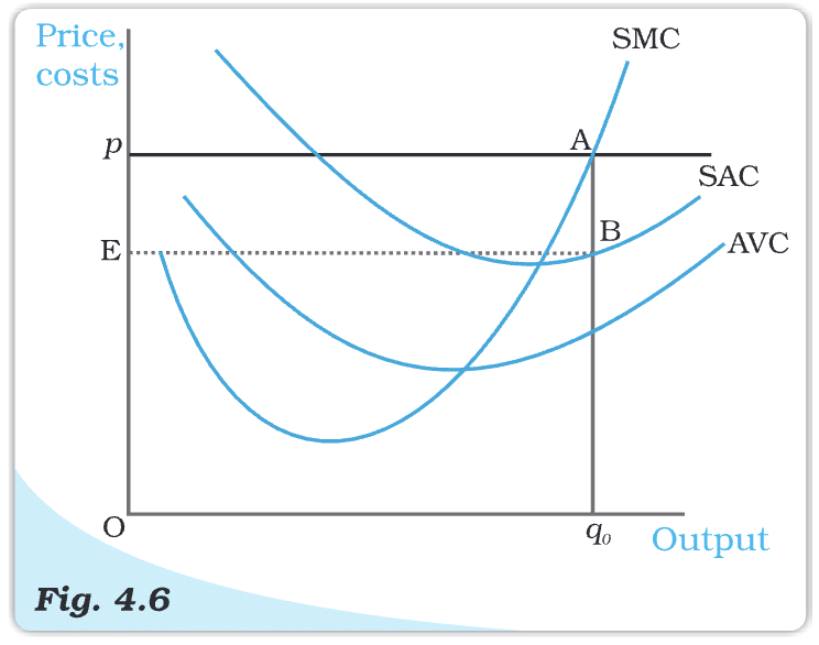
Imagine a firm trying to find the best output level where it can make the most profit. Here's how it works:
- The firm produces at output level q0, where the market price (p) equals the Short Run Marginal Cost (SMC).
- The SMC curve slopes upwards at this point, and the market price (p) is higher than the Average Variable Cost (AVC), which meets all three conditions for profit maximization.
- Total Revenue (TR) at q0 = Area of rectangle OpAq0 (Price × Quantity).
- Total Cost (TC) at q0 = Area of rectangle OEBq0 (Short Run Average Cost × Quantity).
- Therefore, the firm's profit is the area of rectangle EpAB.
The key takeaway? When the price is higher than the cost of producing each unit (SMC), the firm makes a profit.
Question for Chapter Notes - The Theory of the Firm under Perfect Competition
Try yourself:
What does a perfectly competitive market imply about a firm's ability to set prices?View Solution
Supply Curve of a Firm
When we talk about a firm’s supply, we’re simply talking about how much of a product a firm is willing to sell at a particular price. But there’s a catch! This supply is based on three things:
- The price of the product
- The technology available
- The prices of factors of production (like labour, raw materials, etc.)
Supply Schedule:
- A supply schedule is a table that shows the amounts sold by a company at various prices while keeping technology and factor prices constant.
Supply Curve:
- The supply curve of a firm depicts the amounts of output that the firm chooses to create in response to varied market price values while maintaining technology and factor prices constant.
Short Run Supply Curve of a Firm
To figure out how a firm decides its supply in the short run, we need to consider two cases:
Case 1: When Market Price is Greater Than or Equal to Minimum AVC
Imagine the market price is p1, which is higher than or at least equal to the minimum Average Variable Cost (AVC). Here’s what happens:
- The firm looks at where the price line (p1) meets the upward-sloping part of the Short Run Marginal Cost (SMC) curve.
- This point of intersection determines the output level, q1.
- Since the price is higher than the AVC, the firm is covering its variable costs and some of its fixed costs, so it continues producing.
In simpler words, as long as the firm can sell its product at a price that covers its cost of making each extra unit (AVC), it’s in business!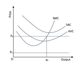
Case 2: Price is less than the minimum AVC
- Presume the market cost price is P2, which is lower than the AVC minimum.
- If a profit-maximizing firm produces a positive output in the short run, the market cost price, P2, has to be higher than or equal to the AVC at that output level.
- The AVC clearly outperforms P2 in the image.
- To put it another way, the company is unable to generate a profit. As a result, if the market price is P2, the enterprise produces no output.
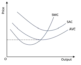
Combining Case 1 and Case 2
Combining both cases gives us a simple but important conclusion:
- The short-run supply curve of a firm is the upward-sloping part of the SMC curve starting from and above the minimum AVC.
- If the market price is below the minimum AVC, the firm’s supply is zero.
 |
Download the notes
Chapter Notes - The Theory of the Firm under Perfect Competition
|
Download as PDF |
Download as PDF
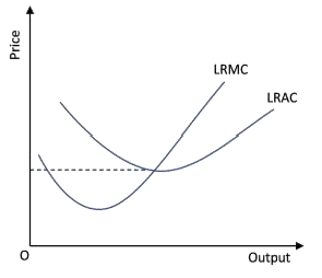
Long-Run Supply Curve of a firm
- When all inputs are variable, the long-run supply is the supply of commodities available.
- The supply curve, in the long run, is always more elastic than the supply curve in the short run.
- In a u-shaped curve, the long-run average cost curve encompasses the short-run average cost curves.
- With the addition of increasing long-run marginal cost curves, the supply curve is upward-sloping.
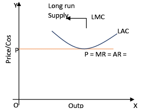
Case 1: Price greater than or equal to the minimum LRAC
- Presume the market cost price is P1, which is greater than the minimum LRAC. We obtain the output degree Q1 by equating P1 with LRMC on the increasing part of the LRMC curve.
- It's also worth noting that the LRAC in Q1 does not exceed the market cost price, P1.
- As a result, at Q1, all three of the conditions are met. When the market cost price is P1, the firm's supplies are equal to Q1 in the long run.
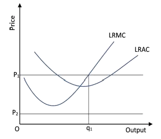
Case 2: Price less than the minimum LRAC
- Assuming the market cost price is P2, which is lower than the LRAC minimum.
- If a profit-maximizing firm produces a positive output over time, the market cost price, P2, must be larger than or equal to the LRAC at that production level.
- In other words, the firm is unable to produce a positive result. As a result, when the market cost price is P2, the firm produces nothing. We reach an important conclusion by combining Cases 1 and 2.
- The long-run supply curve of a business is the increasing section of the LRMC curve from and above the minimum LRAC, as well as the zero production for all-cost prices less than the minimum LRAC.
The Shut Down Point
While deriving the supply curve, we noted that a firm continues to produce in the short run as long as the price is at least equal to the minimum of the Average Variable Cost (AVC). So, as we move down along the supply curve, the last price-output combination where the firm produces positive output occurs where the Short Run Marginal Cost (SMC) curve intersects the AVC curve at its minimum point.
If the price drops below this point, the firm ceases production. This point is known as the short run shut down point of the firm. In the long run, however, the shut down point is determined by the minimum of the Long Run Average Cost (LRAC) curve.
The Normal Profit and Break-even Point
The normal profit is the minimum level of profit needed for a firm to continue operating in the current business. If a firm fails to earn this amount, it won't stay in business. Normal profit is considered a part of the firm’s total costs and can be seen as the opportunity cost of entrepreneurship.
When a firm earns profit above normal profit, it is called super-normal profit.
- In the long run, a firm will not operate if it earns less than the normal profit.
- In the short run, however, the firm may continue producing even if profits are below normal profit.
The point on the supply curve where a firm earns only normal profit is called the break-even point. This occurs where the supply curve intersects the LRAC curve at its minimum point (or the SAC curve in the short run).
Opportunity Cost
In economics, the term opportunity cost refers to the benefit that is given up when choosing one activity over the next best alternative. It represents the potential gain lost from the second-best option that is not chosen.
For example, imagine you have Rs 1,000 and decide to invest it in your family business. What is the opportunity cost of this decision?
- If you keep the money at home, it earns zero return.
- If you deposit it in bank-1, you earn an interest of 10%.
- If you deposit it in bank-2, you earn an interest of 5%.
The best alternative to investing in your family business is depositing the money in bank-1, where you would earn the highest interest of 10%. However, by investing the money in your family business, you lose the opportunity to earn that interest.
Therefore, the opportunity cost of investing the money in your family business is the interest you would have earned from bank-1 (10%).
Question for Chapter Notes - The Theory of the Firm under Perfect Competition
Try yourself:
What determines a firm's supply in the short run?View Solution
Determinants of Supply Curve
In the previous section, we established that a firm’s supply curve is a segment of its marginal cost (MC) curve. Therefore, any factor that influences the MC curve also affects the firm's supply curve.
In this section, we will discuss two important factors that impact the supply curve:
Technological Progress
When a firm uses two factors of production, like capital and labour, to produce a good, a technological improvement (such as an organizational innovation) can enhance productivity. This means:
- More output is produced with the same amount of capital and labour.
- Alternatively, the firm can produce the same amount of output using fewer inputs.
This improvement lowers the firm's marginal cost (MC) at any given level of output, causing a rightward or downward shift of the MC curve.
Since a firm's supply curve is part of the MC curve, technological progress shifts the supply curve to the right.
As a result, at any market price, the firm supplies more units of output.
Input Prices
The prices of inputs (such as wages for labour) also affect a firm's supply curve.
- If the price of an input increases (e.g., higher wage rates), the cost of production rises.
- This increase in cost leads to a rise in both the average cost (AC) and marginal cost (MC) at any output level.
The MC curve shifts leftward or upward, causing the firm’s supply curve to shift to the left.
As a result, at any market price, the firm supplies fewer units of output.
Impact of a Unit Tax on Supply
A unit tax is a tax imposed by the government per unit of output sold. For example, if the unit tax is Rs 2, then a firm producing and selling 10 units of a good must pay a total tax of 10 × Rs 2 = Rs 20.
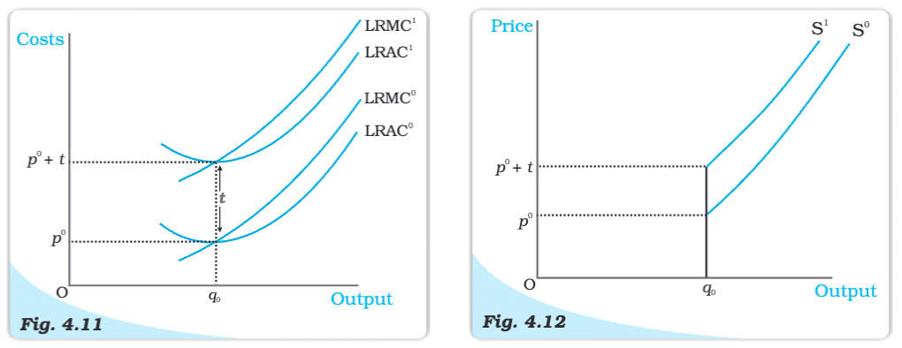
Effect on the Long-Run Supply Curve
When a unit tax is imposed, it increases both the long-run average cost (LRAC) and long-run marginal cost (LRMC) by the amount of the tax (Rs t) at any level of output.
- Before Tax: The firm's LRMC and LRAC are represented by LRMC0 and LRAC0.
- After Tax: With the imposition of the unit tax, the curves shift upward to LRMC1 and LRAC1.
Since the long run supply curve of a firm is the rising part of the LRMC curve above the minimum LRAC, the unit tax shifts the supply curve to the left.
- At any given market price, the firm now supplies fewer units of output.
 |
Take a Practice Test
Test yourself on topics from Commerce exam
|
Practice Now |
Practice Now
Market Supply Curve
The market supply curve shows the total output produced by all firms in a market at different market prices.
How is the Market Supply Curve Derived?
Consider a market with n firms: firm 1, firm 2, firm 3, and so on. If the market price is fixed at p, then the total market supply at that price is calculated by adding up the supply of each firm at that price.
Market Supply = [Supply of firm 1 at price p] + [Supply of firm 2 at price p] + ... + [Supply of firm n at price p].
Geometric Representation (Two Firms Example)
Suppose there are two firms with different cost structures:
- Firm 1 will produce only if the market price is greater than or equal to p1.
- Firm 2 will produce only if the market price is greater than or equal to p2 (where p2 > p1).
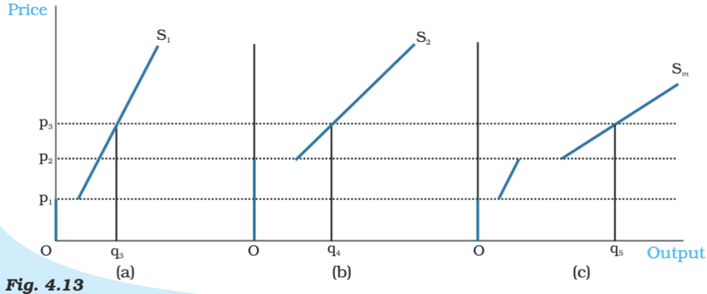
How the Market Supply Curve is Constructed:
When the market price is below p1:
- Neither firm produces anything.
- Market supply is zero.
When the market price is between p1 and p2:
- Only Firm 1 produces.
- The market supply curve coincides with the supply curve of Firm 1.
When the market price is above p2:
- Both Firm 1 and Firm 2 produce.
- The total supply is the sum of the outputs of Firm 1 and Firm 2 at that price.
- The market supply curve is obtained by horizontally adding the supply curves of the two firms.
Understanding Market Supply Curve with a Numerical Example
The market supply curve we derived before assumed a fixed number of firms. When the number of firms changes, the market supply curve shifts:
- If the number of firms increases, the market supply curve shifts to the right.
- If the number of firms decreases, the market supply curve shifts to the left.
Now, let’s look at a numerical example involving two firms.
Supply Curves of the Firms
1. Firm 1's Supply Curve (S1(p))
When p < 10, the firm produces 0 units.
When p ≥ 10, the output produced is (p - 10).
So,
S1(p) = 0 if p < 10.
S1(p) = p - 10 if p ≥ 10.
2. Firm 2's Supply Curve (S2(p))
When p < 15, the firm produces 0 units.
When p ≥ 15, the output produced is (p - 15).
So,
S2(p) = 0 if p < 15.
S2(p) = p - 15 if p ≥ 15.
3. Market Supply Curve (Sm(p))
The market supply curve is the sum of the individual supply curves, i.e.,
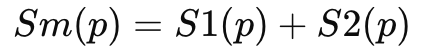
Now, let’s break down the calculation:
- When p < 10: Both firms produce 0 units.
When 10 ≤ p < 15:
- Only Firm 1 produces.

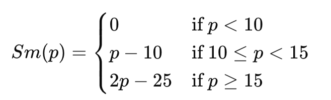
When p ≥ 15:
- Both firms produce.

The market supply curve can be summarised as:
Price Elasticity of Supply
- The price elasticity of supply is a measurement of how sensitive a given good's quantity is to a change in price.
Measurement of Price Elasticity of Supply:
- Price elasticity of supply curve,
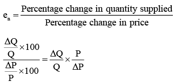
WhereΔQ = change in the quantity of the good supplied to the market
ΔP = change in the price of the good
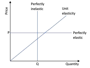
Extreme Cases of Price Elasticity of Supply:
- Perfect elasticity supply (es = ∞): The extreme case of perfect elasticity is when the demanded quantity (Qd) or the supplied quantity (Qs) changes by an enormous amount in response to any change in price. The supply and demand curves are both horizontal in both instances. Ï
- Perfect inelasticity supply (es = 0): If a given quantity of a service or commodity can be supplied at any price, it has a perfectly inelastic supply. The supply elasticity of such a service or commodity is zero. A straight line parallel to the Y-axis is a perfectly inelastic supply curve. This illustrates how supply remains constant regardless of price.
Equilibrium Price:
- It is the point at which the supply of commodities equals the demand.
- When a major index undergoes a period of consolidation or sideways motion, the forces of supply and demand are considered to be relatively equal, and the market is said to be in a condition of equilibrium.
Equilibrium Quantity:
- When there is no scarcity or excess of a product on the market, it is said to be in equilibrium quantity.
- When supply and demand meet, the quantity of an item that customers want to buy equals the quantity that producers are willing to produce.
Application of Demand Supply:
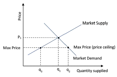
- Maximum Price Ceiling: This refers to the lowest price that sellers are permitted to charge in comparison to the equilibrium market price. When the demand for necessary products exceeds the supply, the government imposes a ceiling. That is, when there are shortages among consumers and the equilibrium price is excessively high. It is done by the government in the benefit of consumers. Rationing and dual marketing may be used to meet excess demand.
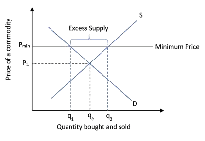
- Minimum Price Ceiling: This means that producers are not allowed to sell their goods below the price set by the government. If the government determines that the equilibrium price is too low for the produce it sets a price ceiling higher than the equilibrium price to protect producers from potential losses. The price is also known as the minimum support price or the floor price. In most cases, the government purchases the extra supply at this price.
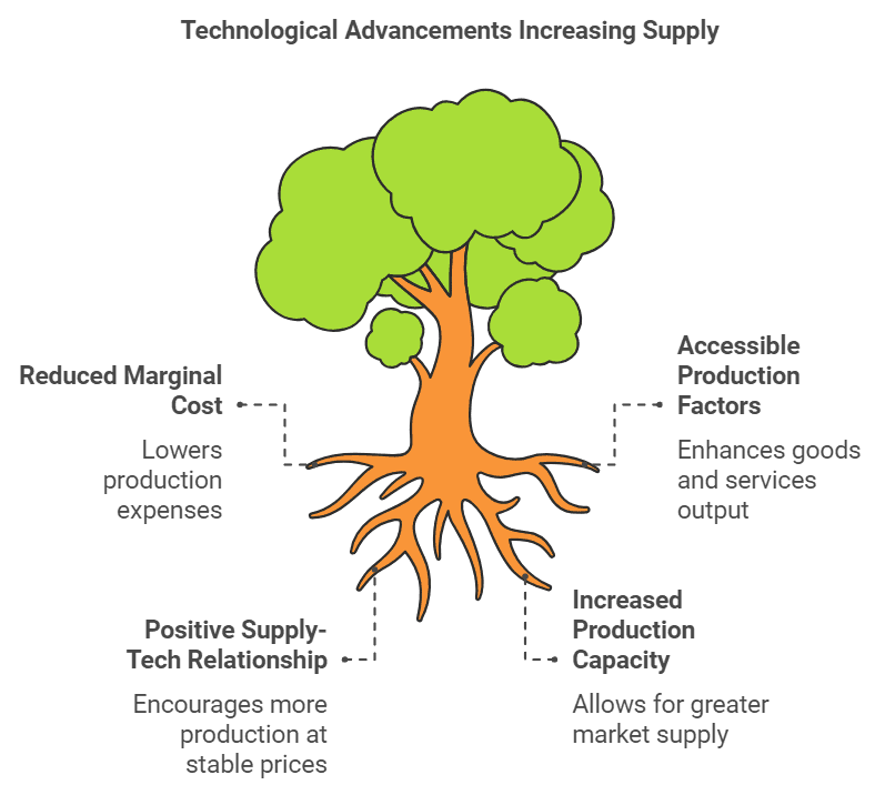
Effect of Technological Advancement on Supply Curve
- The marginal cost of production is reduced as technology advances. With the help of accessible factors of production, producers can generate significantly more goods and services. The supply curve is anticipated to shift rightward and the marginal cost curve is downward because of this circumstance.
- Supply and technical growth have a beneficial relationship.
- Technological advancements frequently result in lower production costs, allowing manufacturers to produce and sell more goods and services at the same price.
- As a result, technological advancement is expected to boost supply, leading the supply curve to shift to the right.
The document Revenue Class 12 Economics is a part of the Commerce Course Economics Class 11.
All you need of Commerce at this link: Commerce
|
58 videos|216 docs|44 tests
|


FAQs on Revenue Class 12 Economics
| 1. What is the market price line in perfect competition? |  |
| 2. How do firms achieve profit maximization in perfect competition? | |
Ans. Firms in perfect competition achieve profit maximization by producing at the output level where marginal cost (MC) equals marginal revenue (MR). Since the price is constant and equal to MR in perfect competition, firms will increase production until the cost of producing one more unit equals the revenue gained from selling that unit. This is the profit-maximizing equilibrium point.
| 3. What is the significance of the profit equilibrium point for firms in a perfectly competitive market? | |
Ans. The profit equilibrium point is significant as it indicates the level of output where firms make maximum profits. At this point, the difference between total revenue and total costs is at its highest. If firms operate at any other level of output, they may either incur losses or have lower profits, making it crucial for firms to identify and maintain this equilibrium.
| 4. Can firms in perfect competition earn long-term profits? | |
Ans. In the long run, firms in perfect competition cannot earn abnormal profits due to the entry and exit of firms in the market. If existing firms are earning profits, new firms will be attracted to the market, increasing supply and driving prices down until profits are normalized. Conversely, if firms incur losses, some will exit the market, reducing supply and pushing prices back up to the point where firms can earn normal profits.
| 5. How does the concept of revenue relate to the market price line in perfect competition? | |
Ans. In perfect competition, the concept of revenue is directly linked to the market price line because firms sell their products at the prevailing market price. Since all firms face the same price, their total revenue (TR) is calculated by multiplying the price by the quantity sold (TR = Price × Quantity). This relationship is essential for firms to determine their output level and assess profitability in relation to costs.
Related Exams
About this Document

4.9K Views

4.96/5
Rating

Mar 26, 2025
Last updated
Document Description: Chapter Notes - The Theory of the Firm under Perfect Competition for Commerce 2025 is part of Economics Class 11 preparation.
The notes and questions for Chapter Notes - The Theory of the Firm under Perfect Competition have been prepared according to the Commerce exam syllabus. Information about Chapter Notes - The Theory of the Firm under Perfect Competition covers topics
like What is a Market?, Perfect Competition: Defining Features, Revenue , Profit Maximisation, Supply Curve of a Firm, Determinants of Supply Curve, Market Supply Curve and Chapter Notes - The Theory of the Firm under Perfect Competition Example, for Commerce 2025 Exam. Find important definitions, questions, notes, meanings, examples, exercises and tests below for Chapter Notes - The Theory of the Firm under Perfect Competition.
Introduction of Chapter Notes - The Theory of the Firm under Perfect Competition in English is available as part of our Economics Class 11
for Commerce & Chapter Notes - The Theory of the Firm under Perfect Competition in Hindi for Economics Class 11 course.
Download more important topics related with notes, lectures and mock test series for Commerce
Exam by signing up for free. Commerce: Revenue Class 12 Economics
Description
Full syllabus notes, lecture & questions for Revenue Class 12 Economics - Commerce | Plus excerises question with solution to help you revise complete syllabus for Economics Class 11 | Best notes, free PDF download
Information about Chapter Notes - The Theory of the Firm under Perfect Competition
In this doc you can find the meaning of Chapter Notes - The Theory of the Firm under Perfect Competition defined & explained in the simplest way possible. Besides explaining types of
Chapter Notes - The Theory of the Firm under Perfect Competition theory, EduRev gives you an ample number of questions to practice Chapter Notes - The Theory of the Firm under Perfect Competition tests, examples and also practice Commerce
tests

Related Searches
shortcuts and tricks
,ppt
,video lectures
,Important questions
,MCQs
,Revenue Class 12 Economics
,mock tests for examination
,Revenue Class 12 Economics
,Semester Notes
,Exam
,Extra Questions
,Viva Questions
,past year papers
,Objective type Questions
,Revenue Class 12 Economics
,practice quizzes
,study material
,Previous Year Questions with Solutions
,Free
,Summary
,Sample Paper
;


Additional Information about Chapter Notes - The Theory of the Firm under Perfect Competition for Commerce Preparation
Chapter Notes - The Theory of the Firm under Perfect Competition Free PDF Download
The Chapter Notes - The Theory of the Firm under Perfect Competition is an invaluable resource that delves deep into the core of the Commerce exam.
These study notes are curated by experts and cover all the essential topics and concepts, making your preparation more efficient and effective.
With the help of these notes, you can grasp complex subjects quickly, revise important points easily,
and reinforce your understanding of key concepts. The study notes are presented in a concise and easy-to-understand manner,
allowing you to optimize your learning process. Whether you're looking for best-recommended books, sample papers, study material,
or toppers' notes, this PDF has got you covered. Download the Chapter Notes - The Theory of the Firm under Perfect Competition now and kickstart your journey towards success in the Commerce exam.
Importance of Chapter Notes - The Theory of the Firm under Perfect Competition
The importance of Chapter Notes - The Theory of the Firm under Perfect Competition cannot be overstated, especially for Commerce aspirants.
This document holds the key to success in the Commerce exam.
It offers a detailed understanding of the concept, providing invaluable insights into the topic.
By knowing the concepts well in advance, students can plan their preparation effectively.
Utilize this indispensable guide for a well-rounded preparation and achieve your desired results.
Chapter Notes - The Theory of the Firm under Perfect Competition
Chapter Notes - The Theory of the Firm under Perfect Competition Notes offer in-depth insights into the specific topic to help you master it with ease.
This comprehensive document covers all aspects related to Chapter Notes - The Theory of the Firm under Perfect Competition.
It includes detailed information about the exam syllabus, recommended books, and study materials for a well-rounded preparation.
Practice papers and question papers enable you to assess your progress effectively.
Additionally, the paper analysis provides valuable tips for tackling the exam strategically.
Access to Toppers' notes gives you an edge in understanding complex concepts.
Whether you're a beginner or aiming for advanced proficiency, Chapter Notes - The Theory of the Firm under Perfect Competition Notes on EduRev are your ultimate resource for success.
Chapter Notes - The Theory of the Firm under Perfect Competition Commerce Questions
The "Chapter Notes - The Theory of the Firm under Perfect Competition Commerce Questions" guide is a valuable resource for all aspiring students preparing for the
Commerce exam. It focuses on providing a wide range of practice questions to help students gauge
their understanding of the exam topics. These questions cover the entire syllabus, ensuring comprehensive preparation.
The guide includes previous years' question papers for students to familiarize themselves with the exam's format and difficulty level.
Additionally, it offers subject-specific question banks, allowing students to focus on weak areas and improve their performance.
Study Chapter Notes - The Theory of the Firm under Perfect Competition on the App
Students of Commerce can study Chapter Notes - The Theory of the Firm under Perfect Competition alongwith tests & analysis from the EduRev app,
which will help them while preparing for their exam. Apart from the Chapter Notes - The Theory of the Firm under Perfect Competition,
students can also utilize the EduRev App for other study materials such as previous year question papers, syllabus, important questions, etc.
The EduRev App will make your learning easier as you can access it from anywhere you want.
The content of Chapter Notes - The Theory of the Firm under Perfect Competition is prepared as per the latest Commerce syllabus.
|
© EduRev
|
Education Revolution
|


|


Signup to see your scores
go up
within 7 days!
within 7 days!
Takes less than 10 seconds to signup