Farm Budgeting - 2 | Agriculture Optional for UPSC PDF Download
Comprehensive Farm Budgeting
This is a method used to gather and organize information about the entire farm, aimed at facilitating decisions concerning the management of farm resources. It strives to estimate all the cost and revenue components, providing a full overview of the farm business. Typically, it is employed by beginners or farmers looking to completely revamp their existing farm structure and operations.
Complete and partial budgeting complement each other, meaning that partial budgeting should be used at various stages within comprehensive budgeting to determine the necessary changes in farm organization.
The process of comprehensive budgeting involves:
- assessing the current farm resources, how they are used, and their efficiency,
- evaluating alternatives, opportunities, and various production activities that can be incorporated, along with their resource requirements, and
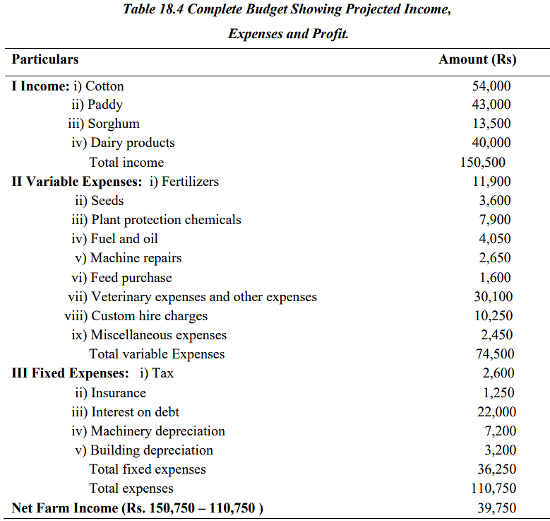
- creating and assessing alternative plans for their feasibility and profitability. The provided table displays an estimated profit or net farm income of Rs. 39,750, assuming that the prices and yields are realized as planned. Any changes in these factors will naturally impact the actual profit generated from operating the farm under this plan.
Applications:
- It serves as a foundation for comparing different plans in terms of profitability, which is particularly valuable when planning for farm growth and expansion.
- An in-depth whole farm budget, indicating the projected profit, can be used to secure the necessary operational capital.
Distinctions between Comprehensive Budgeting and Partial Budgeting:
- Comprehensive budgeting addresses substantial alterations in the farm's structure and operations, whereas partial budgeting deals with minor changes.
- Comprehensive budgeting takes into account all available alternatives, while partial budgeting focuses on just a couple of alternatives.
- Comprehensive budgeting is employed to estimate the outcomes of the entire farm's organization and operation, while partial budgeting is primarily used to assess the net effects in terms of costs and returns resulting from relatively minor changes.
Linear Programming
The simplex method, pioneered by George Dantzig in 1947 for efficient and cost-effective ammunition transportation, is the foundation of linear programming. Linear programming is a mathematical approach that identifies the most favorable or optimal combination of business activities to achieve a specific goal.
To apply linear programming, three key components are essential:
- a goal to either maximize or minimize,
- a range of activities or processes at one's disposal to achieve this goal, and
- a series of constraints or limitations that restrict one's ability to reach the desired objective.
Fundamental Assumptions of Linear Programming:
- Proportionality or Linearity: Linear relationships exist between activities and resources. For instance, if one acre requires 30 man-days, 100 Kgs of nitrogen, and Rs.60 of variable expenses to produce 20 quintals of maize, then 10 acres of maize would need exactly 10 times the resources to produce 200 quintals of output.
- Additivity: The total resources used by multiple farm enterprises must equal the sum of resources used by each individual enterprise, implying no interaction between them. The same applies to the products.
- Divisibility: It's possible to use fractions, and farm enterprises can be produced in fractional units. Resources and products are infinitely divisible.
- Non-negativity: None of the activities can have negative values.
- Finiteness: The number of activities and constraints is finite.
- Certainty: Most planning techniques assume that resources, supplies, input-output coefficients, and prices are known with certainty.
Key Concepts in Linear Programming:
- Solution: A solution denotes any set of activities Xj, j = 1, 2, 3, ..., n, that satisfies a system of inequality constraints. There can be multiple solutions to a given linear programming problem.
- Feasible Solution: Any solution to a linear programming problem is considered feasible if none of the Xj values is negative.
- Infeasible Solution: This term refers to a solution where some of the variables, Xj, have negative values.
- Optimum Solution: Among the feasible solutions, one is considered optimum if such a solution exists. An optimum solution optimizes the objective function, adheres to the constraints, non-negativity restrictions, and maximizes the objective function.
- Unbounded Solution: Occasionally, due to an improperly formulated linear programming problem, it may result in an arbitrarily large value for the objective function, with no finite maximum profit. This scenario represents an unbounded solution in linear programming.
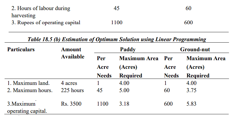
Determining the Optimal Solution through Linear Programming is outlined in Table 18.5.


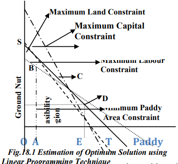
The farmer wants to add an extra condition to the analysis: he requires the farm plan to include a minimum of 0.7 acres of paddy. The area enclosed by the line connecting points A, B, C, D, and E in Figure 18.1 represents all the various combinations of paddy and groundnut that can be cultivated on this farm. This region is known as the feasible production region. Any point outside this line indicates a combination of paddy and groundnut that cannot be achieved without violating one of the constraints.
To complete the graphical analysis, the goal is to determine the optimal mix of paddy and groundnut that maximizes the net return while satisfying the fixed resource constraints of land, labor, operating capital, and the minimum acreage requirement. This is accomplished by establishing a line that represents a constant level of net revenue for different acreage combinations of paddy and groundnut.
The slope of this iso-revenue line can be calculated using the following equation: The farmer's goal is to identify an iso-revenue line that is as distant from the origin as feasible, as this would result in higher net income. Additionally, it is crucial to ensure that this iso-revenue line falls within the feasible production region. The iso-revenue line represented by points S and T meets both of these criteria. Consequently, the production levels indicated at corner point D yield the highest achievable net income.
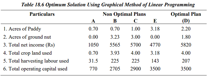
 The best course of action involves cultivating 2.20 acres of paddy and 1.80 acres of groundnut. This plan results in a total net income of Rs. 5620. All 4 acres of cropland and Rs. 3500 in capital are fully utilized, but there are 18 unused labor hours (225 - 207). It's worth noting that suboptimal plans like A, B, C, and E generate lower net income compared to the optimal plan (D).
Drawbacks of Linear Programming:
- Enormous computational challenges may arise (resulting in potentially unbounded solutions).
- Linear Programming does not factor in the element of time.
- Many real-world scenarios are non-linear in nature, whereas Linear Programming exclusively deals with linear equations.
- Applying Linear Programming to macro-level models can be exceedingly challenging. Rounding the variable solutions can significantly change the optimal solution's value.
|
52 videos|224 docs
|


