Inference about population variances | Management Optional Notes for UPSC PDF Download
Testing Hypotheses for a Single Sample
We have previously discussed the concepts of null and alternative hypotheses, as well as the application of z-tests for large samples and t-tests for small samples. In many instances, we are tasked with determining whether a sample significantly differs from a known population. For instance, suppose we conducted a survey of 400 households in the Raigarh district of Chhattisgarh state and calculated their per capita income. Our objective is to assess whether the per capita income derived from the sample differs significantly from that of the entire district.
In such scenarios, two distinct situations may arise: i) when the population variance is known, and ii) when the population variance is unknown to us. Below, we outline the steps to be followed in each case.
Population Variance is Known:
- State the null hypothesis.
- Determine whether a one-tailed or two-tailed test is needed. Accordingly, identify the critical region, aiding in the specification of the alternative hypothesis.
- Apply sample values to the z-statistic.
- Refer to the z-table to find the critical value corresponding to the chosen significance level.
- If the calculated value is lower than the tabulated value, retain the null hypothesis.
- If the calculated value exceeds the tabulated value, reject the null hypothesis and accept the alternative hypothesis.
Example 1: Let us consider the case that we know the per capita income of Raigarh district of Chhatisgarh as well as its variance. Suppose the data available in official records show that per capita income of Raigarh district is Rs. 10,000 and standard deviation of per capita income is Rs. 1,500. However, we did a sample survey of 400 households and found that their per capita income is Rs. 10,500. Do we accept the data provided in official records?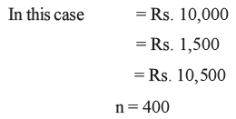
Given a large sample size and known population variance, we utilize the z-test as illustrated in Figure Our null hypothesis, denoted as  , posits that the sample mean equals the population mean. Put differently, it suggests that the per capita income derived from the sample mirrors the data documented in official records.
Our alternative hypothesis is
By substituting values in the above we obtain

In the aforementioned scenario, with z = 6.67, the sample falls within the critical region, leading us to reject the hypothesis. Consequently, the per capita income derived from the sample significantly deviates from the per capita income documented in official records.
Example 2: Consider a scenario where the voltage generated by a particular brand of battery follows a normal distribution. A random sample of 100 such batteries yielded a mean voltage of 1.4 volts. At a significance level of 0.01, does this suggest that these batteries possess an average voltage different from 1.5 volts? It is assumed that the population standard deviation is 0.21 volts.
Here, H0: = 1.5
Since average voltage of the sample can be different from average voltage of the population if it is either less than or more than 1.5 volts, our rejection region is on both sides of the normal curve. Thus it is a case of two-tail test and alternative hypothesis is
Since the population standard deviation s is known, the test statistic is
According to Table 17.2, the critical value at a significance level of 1% is found to be 2.58. Given that the actual value of z exceeds 2.58, we reject the null hypothesis at the 1% significance level and instead accept the alternative hypothesis, indicating that the average life of batteries differs from 1.5 volts.
Population Variance not Known:
It is unrealistic to assume that we know the population standard deviation (σ), as we are typically unaware of the population mean itself. In cases where σ is unknown, we must estimate it using the sample standard deviation (s). Under such circumstances, two possibilities arise based on the sample size. If the sample size is large (n), we utilize the z-statistic.
In case the sample size is small (n 30) we apply t-statistic with n 1 degrees of freedom. The test statistic is
Here are the steps you should follow:
- Define the null hypothesis and alternative hypothesis.
- Determine whether the sample size is large (n ≥ 30) or small (n < 30).
- If the sample size is large (n ≥ 30), apply the z-test (as discussed in Section 17.5).
- Consult the z-table to find the critical value corresponding to the chosen significance level (α).
- If the sample size is small (n < 30), apply the t-test (as discussed in Section 17.6).
- Refer to the t-table to find the critical value for degrees of freedom (n - 1) and the chosen significance level (α).
- If the calculated test statistic is lower than the tabulated critical value, retain the null hypothesis.
- If the calculated test statistic exceeds the tabulated critical value, reject the null hypothesis and accept the alternative hypothesis.
Testing for Differences Between Two Samples
- Frequently, there arises a need to examine the contrast between two samples. The aim might involve determining whether both samples originate from the same population or to check whether a particular characteristic is the same in two populations. For example, we formulate a hypothesis that the production per worker in plant A is the same as the production per worker in plant B. We discuss below the procedure for testing of such a hypothesis.
- Once again, we encounter two scenarios: whether the variances of both populations are known, and another consideration is the sample size: whether it's large or small.
The null hypothesis posits that the population means of both populations are identical. In mathematical notation:
H₀: μ₁ = μ₂ ...
The alternative hypothesis, conversely, suggests that the population means differ:
H₁: μ₁ ≠ μ₂ ...
When the standard deviations (the positive square roots of the variances) of both populations are known, we utilize the z-statistic, which is defined as follows:

In equation above, the subscript 1 pertains to the first sample, and the subscript 2 pertains to the second sample. By inputting pertinent data into equation, we derive the actual value of z and juxtapose it with the tabulated value for the specified level of significance.
Example 1: A bank wants to find out the average savings of its customers in Delhi and Kolkata. A sample of 250 accounts in Delhi shows an average savings of Rs. 22500 while a sample of 200 accounts in Kolkata shows an average savings of Rs. 21500. It is known that standard deviation of savings in Delhi is Rs. 150 and that in Kolkata is Rs. 200. Can we conclude at 1 percent level of significance that banking pattern of customers in Delhi and Kolkata is the same?
In this case the null hypothesis is H0: 1 2
and the alternative hypothesis is HA: 1 2
We are provided with the information that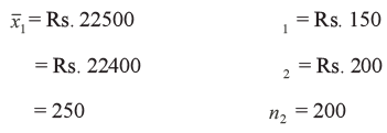
Since 1 and are known we apply z-test.
The test statistic is
By applying the information provided above we obtain
We find that at 1 per cent level of significance the critical value obtained from Table 17.1 is 2.58.
Since the actual value is greater than the tabulated value the null hypothesis is rejected and the alternative hypothesis is accepted. Thus the banking pattern of customers in Delhi and Kolkata are different.
Example 2: A mathematics teacher wants to compare the performance of Class X students in two sections. She administers the same set of questions to 25 students in Section A and 20 students in Section B. she finds that Section A students have a mean score of 78 marks with standard deviation of 4 marks while Section B students have a mean score of 75 marks with standard deviation of 5 marks. Is the performance of students in both Sections different at 1 percent level of significance?
In this case the null hypothesis H: is 1 2
and the alternative hypothesis is H A: 1 2
We are provided with the information that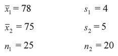
Since 1 and 2 are not known and sample sizes are small we apply t-test.
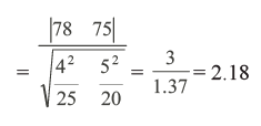
The degree of freedom in this case is 25+20-2 = 43.
We can find out from Table 17.3 that at the 1 per cent level of significance the t-value for 43 degrees of freedom is 2.69.
Since the tabulated value of t is less than actual value of t we reject the hypothesis.
Therefore, students in Section A and Section B are different with respect to their performance in mathematics.
Contingency Table
- The concepts of confidence interval and the procedures of testing a hypothesis discussed so far relate to numerical. In the case of qualitative data, however, we cannot undertake such tests, as we do not have parameters. In the qualitative data, therefore, we require to develop non-parametric tests.
- There are many types of non-parametric tests depending upon our need. However, we confine ourselves to a common procedure, that is, chi-square (pronounced as kaisquared) test for the test of independence between variables. Recall that qualitative data can be arranged in categories (see Unit 6) and presented in the form of a twoway table.
- In order to explain the application of chi-square test let us take a concrete example.
- Suppose we want to test a hypothesis that number of children in a family is independent of the occupation of father. We divide occupation of father into five categories - i) unemployed, ii) unskilled labour, iii) skilled labour, iv) self-employed, and v) professional.
- Similarly we divide families into five categories according the number of children - i) no child, ii) one child, iii) two children, iv) three children, and v) more than three children.
For a sample of 650 families the data obtained is presented in Table 17.3.
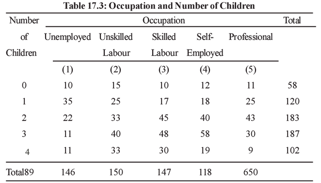
Table 17.3 is called contingency table, because we are trying to find whether the number of children is contingent upon the occupation of the father. Our purpose is test for possible relationship between the number of children and the occupation of father. Thus the null hypothesis is specified as:
- Number of children and occupation of father are independent against the alternative hypothesis
- HA: Number of children and occupation of father are dependent
In Table 17.3 we have presented the observed frequency for each cell in the table.
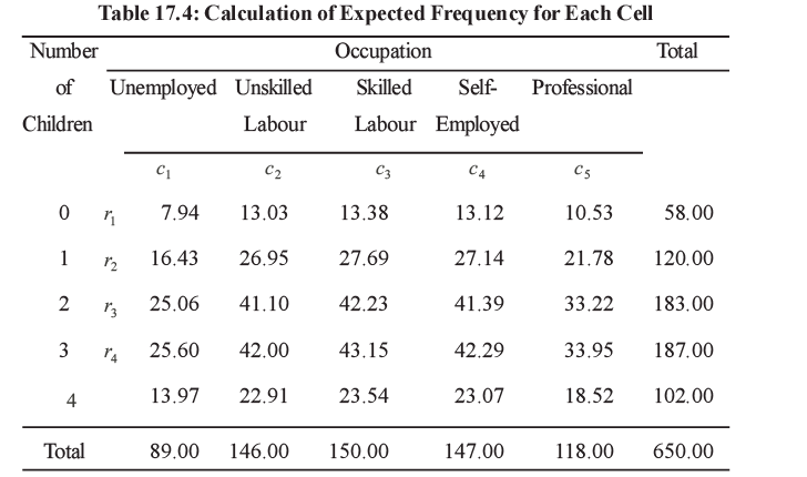
What should be the expected frequency when there is no relationship between the variables under consideration? We will answer this question below. Expected frequency is calculated under the assumption that there is no relationship between number of children and occupation of father. For each cell in Table 17.2 the expected frequency is obtained by

Where Eij is expected frequency for row ‘i’ and column j. For example, for row 2 and column 2 the expected frequency is
We find out the row and column totals for the data given in Table 17.3 and estimate the expected frequency for each cell. These are given in Table 17.4.
The next step is to compare the observed frequency with the expected frequency. In order to compare the observed frequency with the expected frequency we construct the chi-square statistic, which is given by
where O refers to observed frequency and E refers to expected frequency.
The chi-square statistic has degrees of freedom (r 1)(c 1) .
For example, if there are 3 rows and 4 columns, then degrees of freedom is (3 1)(4 1) 6 .
Let us summarise the steps to be followed in chi-square test. These are:
- specify the null and alternative hypotheses
- calculate the expected frequency for each cell by using (20.5)
- Compute the observed value of the statistic using Equation (20.6).
- Determine the degrees of freedom using the formula (r-1)(c-1).Assess the required level of significance (α).
- Calculate the critical value of χ² for the given α and relevant degrees of freedom.
- Compare the observed value of χ² with the critical value of χ².
- If the observed value is less than the critical value, do not reject the null hypothesis (H0).
- If the observed value is greater than the critical value, reject H0 and accept the alternative hypothesis (HA).
- Let's find the observed value of χ² for the data provided in Table 17.4.
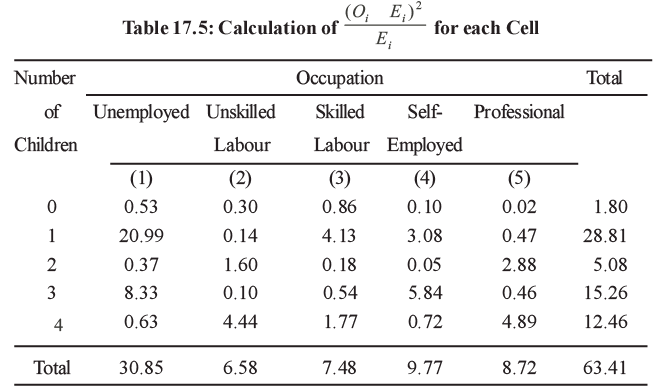
Since there are 5 rows and 5 columns, the degrees of freedom is .
The critical values of x2 for 5% & 1% level of significance for different degrees of freedom are given in Table 17.7 at the end of the Unit. We find from the table that for 16 d.f. the critical value of at 5 per cent level of significance is 26.30. The observed value of 2 to be 63.41. Since the observed value is greater than the critical value we reject the null hypothesis and accept the null hypothesis. Therefore, we conclude that the variables ‘number of children’ and ‘occupation of father’ are not independent.
FAQs on Inference about population variances - Management Optional Notes for UPSC
| 1. What is the purpose of testing hypotheses for a single sample? |  |
| 2. How is testing for differences between two samples useful in research? |  |
| 3. What is the significance of using a contingency table in statistical analysis? |  |
| 4. How does inference about population variances help in research studies? |  |
| 5. What are some commonly asked questions related to hypothesis testing and statistical analysis in exams like UPSC? |  |


