Introduction to probability, Discrete and continuous probability distributions | Management Optional Notes for UPSC PDF Download
Introduction
- Probability, inherently linked with randomness and uncertainty, constitutes a mathematical domain akin to geometry and analytical mechanics. Scholars define probability as the measure of the likelihood of an event occurring, quantified as a number between 0 and 1, where 0 signifies impossibility and 1 denotes certainty. Higher probabilities indicate a greater likelihood of the event happening.
- Probability theory establishes a mathematical framework encompassing concepts such as "probability," "information," "belief," "uncertainty," "confidence," "randomness," "variability," "chance," and "risk." This framework holds significance for empirical scientists, providing them with a cohesive structure to draw inferences and test hypotheses based on ambiguous empirical data. Moreover, probability theory aids engineers in devising systems capable of intelligent operation within an uncertain environment.
- There exist three primary interpretations of probability: the frequentist, the Bayesian or subjectivist, and the axiomatic or mathematical interpretation.
- The frequentist interpretation views probability as the relative frequency of an event occurring over an extended period. In essence, the probability of an event E is interpreted as the proportion of times E is expected to occur in the long run, with this interpretation formalized as the limit of the relative frequency of E's occurrence as the number of observations increases indefinitely.

In this context, "nE" denotes the frequency with which the event is observed out of a total of 'n' independent experiments. This approach to probability holds appeal due to its apparent objectivity, as it establishes a direct link between researchers' endeavors and the observation of tangible events. However, a notable limitation arises from the impracticality of conducting experiments an infinite number of times.
- Probability as Uncertain Knowledge: This conceptualization of probability proves highly advantageous, particularly in the realm of machine intelligence. To function effectively in natural environments, machines require knowledge systems capable of navigating and managing the inherent uncertainty of the world. Probability theory offers an ideal framework for achieving this objective.
- Probability as a Mathematical Model: In contemporary times, mathematicians circumvent the frequentist versus Bayesian debate by treating probability as a mathematical abstraction, divorcing it from specific philosophical interpretations.
- Probability Measures: Typically denoted by the letter 'P' (capitalized), probability measures must adhere to three fundamental constraints, known as Kolmogorov's axioms:
The probability measure of events must be greater than or equal to zero: P(A) ≥ 0 for all events A ∈ F.
- The probability measure of the entire sample space is 1: P(Ω) = 1.
- If sets A1, A2, . . . ∈ F are disjoint, then...

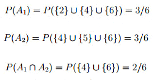
Joint probabilities entail the probability of the intersection of two or more events. For instance, let's examine events A1 = {2, 4, 6} and A2 = {4, 5, 6} within the context of a fair die probability scenario. Here, A1 signifies the event of obtaining an even number, while A2 represents the event of obtaining a number larger than 3.

Thus the joint probability of A1 and A2 is 1/3.
- Conditional Probabilities: The conditional probability of event A1 given event A2 is defined as follows:

- Mathematically this formula amounts to making A2 the new reference set, i.e., the set A2 is now given probability 1 since

- Conditional probability involves adjusting the original probability measure P to account for the occurrence of event A2 with certainty (probability 1).
- The Chain Rule of Probability, also referred to as the general product rule in probability theory, facilitates the calculation of any element within the joint distribution of a set of random variables solely through conditional probabilities. This rule proves advantageous in the analysis of Bayesian networks, which define probability distributions based on conditional probabilities.
- Consider a collection of events (A1, A2, ..., An). The chain rule of probability provides a practical method for computing the joint probability of the entire collection:
- P(A1∩A2∩...∩An)=P(A1)P(A2│A1)P(A3│A1∩A2)...P(An│A1∩A2∩...∩An−1)
- The Law of Total Probability serves as a fundamental principle connecting marginal probabilities to conditional probabilities, elucidating the comprehensive probability of an outcome across various distinct events.
- Bayes' Theorem, credited to Bayes (1744-1809), elucidates the adjustment of event probabilities based on new data. While widely acknowledged within probability theory, this theorem sparks debate among frequentists and Bayesian probabilists regarding its applicability to subjective or frequentist notions of probabilities.
Mathematically, Bayes' theorem is expressed as follows:

In the context where A and B represent events:
- P(A) and P(B) denote the probabilities of events A and B independently of each other.
- P(A | B), a conditional probability, signifies the probability of event A given that event B has occurred.
- P(B | A) denotes the probability of event B given that event A is true.
Discrete and Continuous Probability Distributions
- Probability distributions fall into two main categories: discrete probability distributions and continuous probability distributions, depending on whether they define probabilities for discrete or continuous variables.
- A discrete distribution describes the probability of each value of a discrete random variable. Such a random variable takes on countable values. Each possible value of the discrete random variable in a discrete probability distribution is associated with a non-zero probability. Typically, a discrete probability distribution is presented in tabular form. If the random variable associated with the probability distribution is discrete, it is termed as a discrete distribution. This distribution is characterized by a probability mass function (ƒ).
There are five types of discrete distributions:
- Binomial Distribution: Probability of exactly x successes in n trials.
- Negative Binomial: Probability that exactly n trials are needed to produce x successes.
- Geometric Distribution: Probability of exactly n trials to produce one success (a special case of the negative binomial).
- Hypergeometric Distribution: Probability of exactly x successes in a sample of size n drawn without replacement.
- Poisson Distribution: Probability of exactly x successes in a "unit" or continuous interval.
On the other hand, a continuous distribution defines the probabilities of possible values of a continuous random variable. This type of random variable has an infinite and uncountable range of possible values. Unlike a discrete probability distribution, the probability of a continuous random variable taking on a specific value is zero. Consequently, a continuous probability distribution cannot be represented in tabular form. Instead, it is described by an equation or formula known as a probability density function (PDF).
All probability density functions adhere to the following conditions:
- The random variable Y is a function of X, denoted as y = f(x).
- The value of y is greater than or equal to zero for all values of x.
- The total area under the curve of the function equals one.
It is worth noting that a discrete random variable has distinct boundaries between its different outcomes, whereas a continuous random variable lacks distinct boundaries between outcomes.
FAQs on Introduction to probability, Discrete and continuous probability distributions - Management Optional Notes for UPSC
| 1. What is the difference between discrete and continuous probability distributions? |  |
| 2. How are probabilities assigned in discrete probability distributions? |  |
| 3. What are some common examples of discrete probability distributions? |  |
| 4. How are probabilities assigned in continuous probability distributions? |  |
| 5. What are some common examples of continuous probability distributions? |  |


