Linear Programming: Sensitivity Analysis | Management Optional Notes for UPSC PDF Download
Introduction
Following the resolution of a linear programming problem, it proves beneficial to examine how alterations in the problem's parameters affect the existing optimal solution. Common scenarios involve assessing the effects of changes in profit or cost within the objective function of the current solution, or variations in resource levels affecting the current product mix composition. This investigation can be conducted using the final simplex table and is referred to as sensitivity analysis or post-optimality analysis. We will demonstrate this approach through an example.

Example: We consider the linear programming problem introduced in Section 4.4 Maximise 12X1 + 3x2 + x3
The final simplex Table presenting the optimum solution '(x4, x5, x6 being the slack variables) is presented below :

Change in the Profit coefficient
i. Non-Basic Variable: The variable x3 nonbasic. If its profit level is increased to C3 then the solution remains unchanged so long as

If C3 >116 then the present solution is no longer optimum; A new round of simplex computation is to be performed in which x3 becomes a basic variable; However, if C3 < 1 16, the present solution remains optimum.
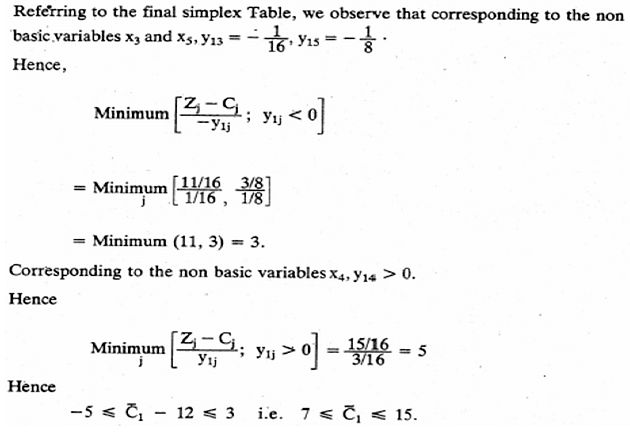
ii. Basic Variable: In this case, the changes can be both positive and negative, as in either case the current solution may become non-optimal. Let us consider the basic variable x1.

Thus the optimal solution is insensitive so long as the changed profit coefficient C1 is between Rs. 7 and Rs. 15 although the present profit coefficient is Rs. 12. Of course, the value of the objective function has to be revised after introducing the change value C1.
FAQs on Linear Programming: Sensitivity Analysis - Management Optional Notes for UPSC
| 1. What is linear programming and how does it relate to sensitivity analysis? |  |
| 2. What is the purpose of sensitivity analysis in linear programming? |  |
| 3. How is sensitivity analysis performed in linear programming? |  |
| 4. What are the limitations of sensitivity analysis in linear programming? |  |
| 5. How can sensitivity analysis benefit decision-making in linear programming? |  |


