Time series and forecasting - 1 | Management Optional Notes for UPSC PDF Download
Introduction
- Forecasting is a crucial tool in predicting future conditions, whether it's anticipating the weather or estimating the potential damage from natural disasters for government planning purposes. In this unit, we'll focus on forecasting quantitative aspects, such as monetary damage or required food-grain quantities.
- The characteristic of interest, which we aim to forecast, is typically influenced by various factors like economic conditions, technology, population, inflation, weather, and seasonal variations. Identifying all these factors may not always be feasible, so instead, we rely on studying the behavior of the characteristic over time to forecast future values. Forecasting methods generally involve two steps: analyzing the historical pattern of the data and extrapolating this pattern into the future. The accuracy of these forecasts heavily relies on correctly identifying patterns and the assumption that these patterns will persist into the future.
- In many cases, it's reasonable to assume that the underlying pattern will remain unchanged, at least in the short term. However, such assumptions may lead to errors in the long run. These forecasting errors can be evaluated by comparing actual values with predicted values, allowing for adjustments in future forecasts.
- We'll explore the utility of forecasting and how to calculate forecasting errors through a practical example.
Example 1: A grocery shop owner in a small colony gets 50 bread loaves every morning from a company and sells them to the residents of that colony. If he sells a loaf, he makes a profit of Rs.2/-. If a loaf is not sold on the same day, the shop owner returns it to the company the next morning but he loses Re. 11- on each loaf returned. In order to maximise his profits, the shop owner decided to study the pattern of the demand for the bread. (The daily demand for bread can be thought of as a random variable.) He collected the data shown in Table 1.
Table: No. of Bread Loaves Demanded
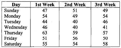
Let us now analyse this data. If we compute the average number of loaves that can be sold per day (that is, the demand per day) based on the three weeks' data, it comes to 50.66 loaves (= average of the 21 numbers in Table I). In fact, from his past experience the shop owner found that he can sell approximately 50 loaves <n an average. This is why he takes 50 loaves every morning from the company for selling. So, based on the data gathered for 3 weeks, the owner's forecast for each day's sale is 50. Let us now compute the forecasting errors (for the owner's forecast) during the first 2 weeks (see Table 2). Table 2: Forecasting Errors For The First Two Weeks

To assess your understanding of the discussion thus far, please attempt the following exercise now.
Calculate the forecasting errors for the third week.
Referencing Table 2, on Sunday of the first week, the shop owner had to return 3 loaves, resulting in a loss of Rs. 31. Additionally, on Monday of the first week, he fell short by 4 loaves, which would have yielded an extra profit of Rs. 81. Therefore, this shortage should also be considered a loss due to his decision to only stock 50 loaves daily. Consequently, the owner's profit on Sunday of the first week amounts to (47 loaves sold × Rs. 2 profit per loaf) - (3 loaves returned × Rs. 1 loss per loaf) = Rs. 91. Similarly, his profit on Monday of the first week equals (50 loaves sold × Rs. 2 profit per loaf) - (4 loaves short × Rs. 2 profit per loaf) = Rs. 92. By extrapolating this method for the entire three weeks, the overall profit totals Rs. 18,321. Do you believe the owner could make better decisions to increase his profit? This might be achievable by improving the accuracy of sales forecasts. How can the owner enhance his forecasting method to minimize forecasting errors? To address this, let's revisit the data from Table 1. Plotting each week's data on a graph with the x-axis representing the days and the y-axis representing the demand yields Fig..
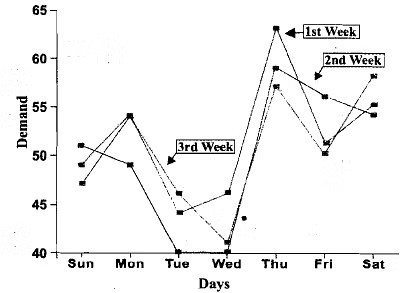
Fig.: Demand of bread loaves vs. days.
(i) The demand fluctuates daily;
(ii) On Tuesdays and Wednesdays, demand is lower compared to other days;
(iii) Thursdays exhibit notably higher demand. It's noteworthy that daily demand is a random variable dependent on time, and its future expected values rely on past observations.
Considering these observations, wouldn't it be prudent for the owner to forecast demand separately for each day of the week and then make decisions accordingly? How could this be achieved? One approach is to forecast each day's demand as the average of the three observations for that day. For instance, the forecast for Sunday's demand would be the average of 47, 51, and 49, resulting in 49. Similarly, Monday's forecast would be the average of 54, 49, and 54, yielding 52.3. Since the number of loaves cannot be fractional, the owner may opt to procure 52 loaves (rounded to the nearest integer). Consequently, the shop owner might decide to acquire 49 loaves on Sundays, 52 on Mondays, and so forth.
Now, let's assess the benefits if the owner adopts this forecasting approach through the following exercise:
Exercise 2: Compute the forecasts for Tuesday to Saturday as described above. Record the forecast errors for the three weeks and compare them with those from Table 2. What is the profit over three weeks according to the new decision?
Having completed Exercise 2, you'll find that the revised forecasting method leads to a profit of Rs. 20,151, while the profit from the previous forecasting method was Rs. 18,321. Therefore, the method discussed above is superior to the former one.
The example provided serves to illustrate the essence of forecasting—how it aids decision-making, understanding forecasting errors, and their computation. In practice, producing highly accurate forecasts may pose challenges due to data not conforming to mathematical models and sudden changes in data patterns. Nonetheless, there are methods to make reasonable forecasts. In the subsequent sections, you'll explore how forecasting models are constructed and the various elements involved in their development.
Time Series
- In the preceding section, you've observed examples demonstrating how data amassed over time can facilitate forecasting. It's evident that forecasting entails analyzing the trajectory of a characteristic over time and scrutinizing the data for discernible patterns. Subsequently, forecasts are formulated under the assumption that the characteristic will persist in accordance with the same pattern in the future. The data collected may pertain to various characteristics such as weekly sales, daily output units, monthly operational costs of a company, and so forth.
- Any data gathered regarding a characteristic over consecutive time intervals is referred to as a time series. For instance, Table presented a day-to-day time series for bread demand. Some time series span across several years, such as the Andhra Pradesh government's investigation into changes in crop patterns over a multi-year period.
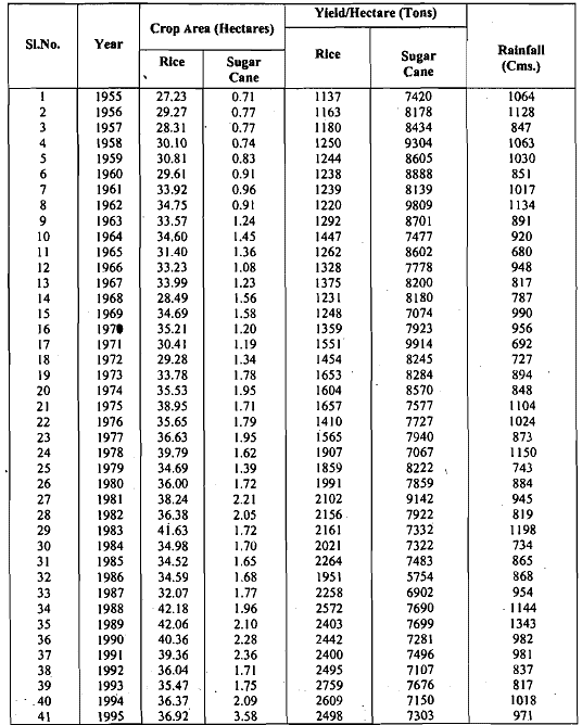
- The predict the fbture economic needs of the agricultural sector. For this purpose, they gathered the pertinent data, some of which are given in Table below.
Table: A Time Series for Crop Yield
 In the preceding section, you've encountered instances illustrating how data amassed over time can facilitate forecasting. It's evident that forecasting involves analyzing the trajectory of a characteristic over time and scrutinizing the data for discernible patterns. Subsequently, forecasts are formulated under the assumption that the characteristic will persist according to the same pattern in the future.
- The data collected may pertain to various characteristics such as weekly sales, daily output units, monthly operational costs of a company, and so forth. Any data gathered regarding a characteristic over consecutive time intervals is referred to as a time series. For instance, Table 1 presented a day-to-day time series for bread demand. Some time series span across several years, such as the Andhra Pradesh government's investigation into changes in crop patterns over a multi-year period.
- These constitute the fundamental elements of any time series upon which forecasting models are constructed. Let's delve into each of these components individually.
Long-term Trend
Take a glance at the data depicting the yield of rice in Table. These data are visually represented in Figure.
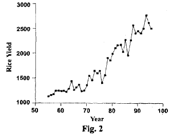
From the graph, it's evident that there's a general upward trajectory in the yield over a span of 40 years, despite occasional downward fluctuations. This upward trend could be attributed to advancements in methods and facilities, the adoption of new rice breeds, and similar factors. Indeed, many business and economic indicators display upward trends over extended periods. However, there are also instances of series exhibiting downward trends. For example, the data on sugar cane yield illustrated in Table depicts a declining trend. Another instance is the mortality rate of children under 10 years old in India (refer to Figure), which demonstrates a pronounced downward trend over a significant duration.
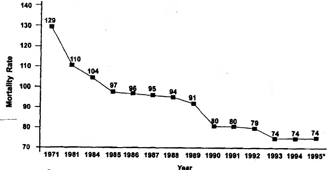
Fig: Infant mortality rate per 1,000 live births In India
Forecasting and Time Series Analysis
Some characteristics do not exhibit any discernible trend over a 15-year period or even longer. For instance, in Figure 4, we visually represent the rainfall data from Table 3. Can you observe any overarching upward or downward trend in it? In time series where no trend is apparent, the long-term trend component will be absent in the forecasting models utilized for such time series.
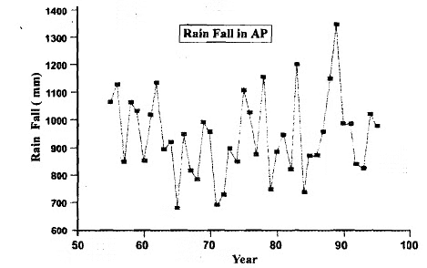
Fig: Example of a time series with no trend So, we have just seen examples of the long-term trend, which is an upward (or downward) movement in a time series over a long period of time, usually 15 years or a longer peiiod.
Seasonal Variations
- Suppose a readymade garment's manufacturer wants to forecast the sales of cotton shirts. He studies the data he has for the period 1995-2000. This data is of quarterly (i.e., 3-monthly) sales, which are given in Table
Table: Quarterly Sales of Cotton Shirts

- Let us draw the graph of these sales by the quarter (see Fig ) for 3 years. From Fig you can see that for each year the sales are low in the first and fourth quarters, but high, and more or less the same, in the second and third quarters. So, within a year, the pattern is different in different quarters.
- However, the same pattern repeats every year. We have shown the sales for only 3 years in Fig. 5. The sales for the other years follow the same pattern. This kind of repetition of a pattern within a time period (of a year in this case), and repeated every year is an example of a seasonal variation.
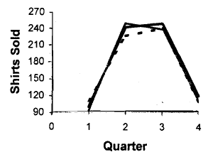
Fig: Quarterly sales of shirts
- In a broader sense, a seasonal variation of a characteristic refers to a recurring pattern observed in the data over a specific time period (such as a year in the aforementioned example), wherein the shape of the pattern repeats in each successive period (as in the example, year after year). For instance, if you examine the data regarding annual rainfall in India, categorized month-wise, you'll notice higher rainfall during July and August, and minimal rainfall during April and May.
- Seasonal variations may not solely stem from changes in natural weather conditions; they can also result from human-made factors. For instance, the number of STD phone calls made during a day may fluctuate based on the time slots designated by the telephone department (currently, MTNL offers two time slots with varying charges). Similarly, the volume of passengers traveling in city buses typically decreases on Saturdays and Sundays compared to other weekdays.
As you may have noticed, seasonal variation significantly influences planning or forecasting, particularly over short periods like a year or less. However, there exists a somewhat analogous component within a time series that, in a way, aligns with the long-term trend.
Cyclic Variations
- When you were studying the data in Table 3, you may have noticed that the data on crop area of sugar cane presented there seems to increase and decrease repeatedly over the 4 1 years. In Fig.6, we present the same data graphically.
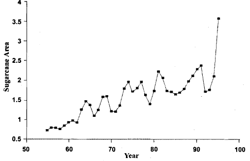
Fig: The crop area of sugar cane in Andhra Pradesh from 1955-1995
- Observing the graph above, it's evident that the crop area experiences fluctuations, initially increasing to a certain point, then declining, followed by subsequent increases and decreases. This type of movement within a time series is termed cyclic variation. A cycle in a time series spans from one peak to the next (or from one lowest turning point to the next), as illustrated in Fig.
- Unlike seasonal variation, the duration of a cycle in cyclic variation is not periodic, as depicted in the graph. For instance, one cycle spans from 1962-66, while another extends from 1966-71, demonstrating varying lengths. Some time series may lack any cyclic variations. Consider, for instance, the time series of child mortality in India depicted in Fig., which exhibits no cyclic component. C
- yclic variations are prevalent in commercial and economic time series, with cycle lengths ranging from 2 to 10 years. While both cyclic and seasonal variations exhibit peaks and troughs, the duration of a seasonal variation is typically short, usually lasting a year or less. Hence, the generally accepted convention is to classify a variation as cyclic only when its duration exceeds a year, whereas a variation lasting a year or less is considered seasonal.
Now we shall britfly consider the fourth component of a time series.
Irregular Variations
- Let's imagine I'm analyzing trends in male versus female birth rates in North India. While examining the annual figures per thousand from 1973 to 2000, I notice a distinct pattern - the number of female births is steadily decreasing. However, this pattern is abruptly disrupted at one point (in 1997) when the number of female births suddenly increases before returning to the previous trend.
- Such unexpected fluctuations in a time series are termed random variation or irregular variation. They stem from one or more chance factors that are entirely random and unpredictable. Therefore, this factor is characterized by a random variable, with its values essentially representing estimates of forecast errors. Consequently, it's anticipated that this variable follows an independent and identically distributed (i.i.d.) normal distribution with a mean of 0. As a result, irregular variation is typically disregarded in long-term planning and forecasting endeavors.
FAQs on Time series and forecasting - 1 - Management Optional Notes for UPSC
| 1. What is time series forecasting? |  |
| 2. What are the key components of a time series? |  |
| 3. What are some commonly used time series forecasting methods? |  |
| 4. What is the role of forecasting in decision-making? |  |
| 5. How can time series forecasting be used in financial markets? |  |


