Time series and forecasting - 2 | Management Optional Notes for UPSC PDF Download
Forecasting Models
- In this section, the key issue we shall discuss is that of appropriate models which explain the available time series data reasonably well. We shall restrict our discussion to two commonly used forecasting models — the additive model and the multiplicative model. While doing so, we shall use the notation yt for the value of the time series at the time t. Since all time series will be in chronological order (i.e., in order of successive time periods), we can use serial numbering for time t. For example, for the
- In the data provided in E8 (iii) (Table 5), we can utilize the time indices t = 71, 72, ..80, where the corresponding time series values would be y71 = 29.9, y72 = 26.7, and so forth. Alternatively, we can serialize this data using indices t = 1, 2, ..., 10, where 1 corresponds to 71, 2 to 72, and so on. In this case, the time series values would be y1 = 29.9, y2 = 26.7, and so on.
Now, let's examine the models individually.
The Additive Model
- One of the most commonly employed models is the additive forecasting model. In this model, it's assumed that at any time t, the time series comprises the sum of all its components. Symbolically, the model is represented as:
yt = Tt + Ct + St + It - Here, Tt, Ct, St, and It denote the long-term trend, cyclic, seasonal, and irregular variations, respectively. Additionally, it's assumed that the effect of the cyclic component (Ct) remains constant across all cycles, and the effect of any seasonal variation (St) remains consistent throughout each year (or corresponding period). Similarly, it's assumed that the irregular component (It) maintains the same effect throughout. (In essence, it's assumed that It follows an independent and identically distributed normal distribution with a mean of 0)
- As illustrated in Sec. , it's not mandatory for every time series to encompass all four components. For instance, the model for the annual rice yield data lacks a seasonal component, while the model for the annual rainfall data doesn't incorporate a cyclical component.
Let's consider an example to demonstrate the application of the additive model.
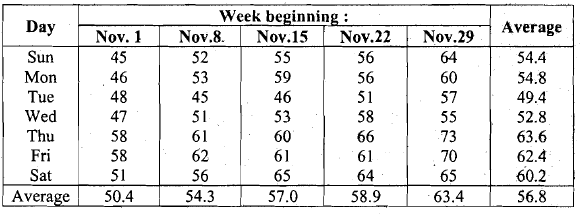
Example 3: Let's revisit the scenario outlined in Example 1. To fit the model, we utilize fresh data gathered during five weeks in November and December 1998, concerning these sales. These data are presented in Table below.
The Multiplicative Model
- We briefly outline this method, which is really a multiplicative version of the earlier one. In the additive model, we have assumed that the time series is the sum of the trend, cyclical, seasonal and random components* From practical experience, scientists have found that additive models are appropriate when the seasonal variations remain unchanged (that is, the seasonal variations do not depend on the trend of the time series).
- However, in practice, there are a number of situations where the seasonal variations change over time, as you will see in Example 4 below. When the seasonal variations exhibit an increasing or decreasing trend, we can try the multiplicative model. In the multiplicative model it is assumed that the time series is obtained as a product of the four time series components, that is,
yt = Tt.Ct.St.It. - Multiplicative models are found to be appropriate for many economic time series data such as data related to production of electricity, number of passengers going abroad, consumption of cold drinks, etc. In the following example, we will briefly describe the application of this model.
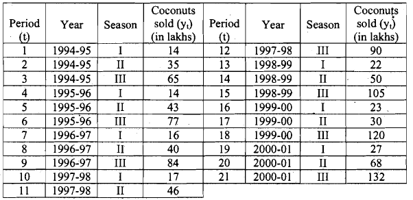
Example 4: Examine the data on coconut sales in Hyderabad from 1995 given in Table 9. In each year, the number of coconuts sold are recorded for three seasons: (i) Season I - March to June, (ii) Season II - July to October, and (iii) Season III - November to February.
Table: Coconut Sales Data
First, let us observe the time series plot. This is given in-Fig. 7.
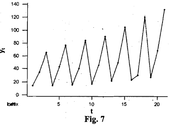 From the plot you can easily see two things:
- the sales are gradually increasing (this indicates the increasing trend), and
- the seasonal variation clearly exists, and, more importantly, it is increasing with the increasing trend.
While doing El 1, you would have realised that the seasonal variation is increasing with an increasing trend. So, as we said at the beginning of this sub-section, we should try the multiplicative model in this case. The cyclic variation that you see in Fig. is actually seasonal variation. . So, we drop the cyclic component Ct, and include the seasonal component S( in our model. Consequently, our model will be :
yt = Ttstit.
- We will see how we can estimate the time series components Tt, St and It, using formal methods, in the next section.
* * * - Note that in order to apply the multiplicative model the time series should-have positive values. So, if we wish to use the multiplicative model to understand a time series with negative values, then we need to convert the time series to positive values by adding a suitable constant to each entry.
- In this section you have seen examples of building forecasting models in some cases. Our approach was an ad hoc one, based on common sense. However, this is not the way analysts do it. In the next section you will learn some scientific methods of analysing time series data.
Forecasting Long-Term Trend
In this section, we employ the least squares method, the moving average method, and the method of exponential smoothing to determine the component Tt mentioned in the models above. Identifying the trend in a time series necessitates the elimination of other components from the time series.
The Least Squares Method
Let's revisit the bread sales data provided in Table. The data is reorganized day-wise in Table 10 for better clarity.
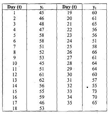
- Now, what do you expect its trend component to be like? Does the trend component of the time series increase (or decrease) at a constant rate? If it does, then the time series is said to have a linear trend, that is, it is a linear function of time. What this means algebraically is that if yt has a linear trend, then we would expect Tt = a + bt, where a and b are constants.
- Recall how you fit linear equations. We can use the method of least squares. Here Tt is our dependent variable and t is our independent variable. Setting y = Tt and x = t, we get
 Therefore, the parameters a and b of the best fit linear equation are estimated as
b = Sxy/Sxx = 0.485, and
a = y-bx = 48.06.
So, the regression equation in this case is given by
Tt = 48.06 + 0.485t. (1)
This equation can now be used to obtain the trend component Tt.
- If you work out the square of the correlations coefficient, you will find R2 = 0.49. From Unit 9, you know that this means that this regression is reasonably reliable, but could be better.
- Notice that in our earlier approach in Example 3, we had the same value for the trend component during any day of the week. In this regression approach, we get different values of the trend even within a week. In the following exercises we ask you to compare some of these different trend values.
Not all datasets display a linear trend. Sometimes, upon observing the data points, it becomes evident that the time series data show non-linear trends. For instance, upon examining the rice yield data depicted in Fig., there's a distinct indication of a non-linear trend.
Table : Andhra Pradesh Population
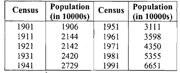
Look & the graph of the time series above given in Fig. below. The points are certainly not lying around any line. Some non-linear curve may fit the data very well.
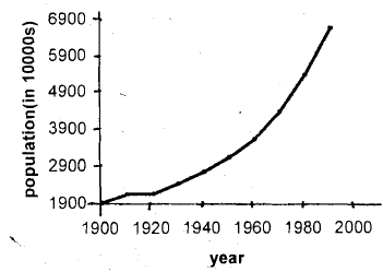
A number of standard forms of curves have been found to be useful for fitting the data, in practice. These are polynomial curves, exponential curves and growth curves. The graphical plots of the time series is useful in identifying the form of the trend curve.
The Method of Moving Averages
- This method aims at identifying the long-term trend by eliminating seasonal variations. While doing this, the method also indicates the presence of seasonal and cyclic variations, if any. To appreciate this, let us apply this method to our bread sales data presented in Table. Example 1 (Contd.): To apply the method we need to present the data in a single column (in chronological order). This is done in Column 2 of Table below.
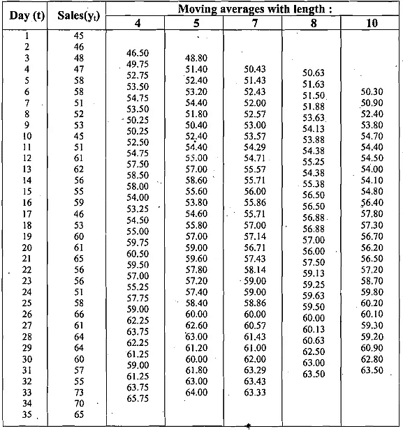
- For now, disregard Columns (3), (4), (6), and (7) in the table. Let's focus on how we obtained the entries in Column (5). Initially, we calculate the average of the first seven observations in Column (2),
 which yields 50.43. This value is placed in Column (5) corresponding to Day 4, representing the mean of Days 1 to 7. Subsequently, we compute the average of the seven observations from y2 to y8, excluding y1 and including y9, resulting in a value of 51.43. This is inserted into Column (5) corresponding to Day 5. This process continues, calculating the averages of seven consecutive observations by excluding the first and including the next, until the last entry in Column (5), 63.33, which represents the average of the final seven observations in Column (2) and is placed alongside Day 32. These computed averages are referred to as moving averages of length 7.
 - Moving on to Column (4), it comprises the moving averages of length 5. Therefore, the initial entry is calculated as
 . This value is placed in line with Day 3. The next entry in Column (4) is in line with Day 3. The next entry in Column (4) is
  and so on.
 - ' We have just seen how to find moving averages of odd length (7 and 5, respectively). Let us now see how to compute the moving averages of even length. Suppose we wish to compute the moving averages of length 4 for the bread sales data. We compute the average of the first 4 observations of Column (2) in Table 14. This average is equal to 46.5. What day does it correspond to? We imagine that it corresponds to 'Day 2.5' (i.e.,
 and place it in Column (3) at the point between the rows 4 corres onding to Day 2 and Day 3. Next, we compute the average of the 2nd,3 ' !,4' and 5' observations. This is 49.75.
 - Correspond this with 'Day 3.5' in Column (3). Since 465 corresponds to Day 2.5 and 49.75 corresponds to Day 3.5, the aierage of 46.5 and 49,75 = (46.5 + 49.75)/2 = 48.125 should correspond to Day 3 (= average of 2.5 and 3.5). In this way we continue, the last entry in Column (3) being
 = 65.75. This is placed in line with 'Day 33-5'. You should calculate and check for yourself that all the entries shown in Columns (3) to (7) are correct.
 - Now let us see the graphic representation of the moving averages. In Fig. 10, we have plotted the mwing averages (of length 7) computed in Column (5), Tablel4, against the corresponding day numbers. The straight line trend obtained in Sec.lO.S.1 (Equation (1)) is also drawn in the figure.
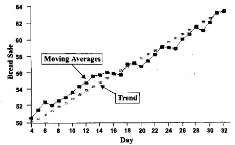
Fig.: Plot of moving averages and linear trend for bread sales data
- Now look at Fig. , where the moving averages of lengths 4,8 and 10 (shown in Table 14) are plotted along with the trend line.
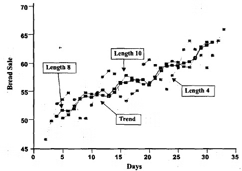
- This is not surprising as the bread sales data have the seasonal component, the season being the seven days of the week. Observe from Fig that approximately half of the moving averages are above the trend line and the rest are below or on the trend line. This is to be expected whenever the linear trend is the best fit, since it represents the 'average' in a sense. If you go back to Fig., you will notice that the time series shown in it doesn't seem to show a linear, quadratic or exponential trend. In fact, it is a very jerky graph. But, related to the same data, Fig. shows us that the moving averages of different lengths of the same data gives us smoother curves that show the long-term movements of the series. In this way the moving averages can be used to estimate the trends, if the time series does not help us in doing so.
* * * - From the example above, can you see what the basic idea is of using moving averages? If the time series of the data contains certain seasonal or cyclical variations, the effect of these variations can be eliminated by taking a moving average where the time period in the average equals the period of the season or the cycle. By smoothening the curve in this way, the trend doesn't get affected. For instance, in the example above the cycle is of length 7 and so the moving averages of length 7 will help us study the long-term trend, since the St-component of y, gets removed.
Before concluding this subsection on the moving averages (MA) method, let's highlight the following points:
- When dealing with a time series that consists of a purely random sequence of numbers, applying a moving average to it often results in showing cyclical fluctuations. This occurrence is due to the serial correlation inherent in a moving average. Hence, it's essential to be aware that many cycles apparent in moving averages might be spurious.
- The peaks and troughs observed in the moving average may not align with those in the original time series.
- It's impractical to compute a moving average for the earliest or latest years in a time series since the computation depends on data that precede or succeed these years.
- The moving averages method is particularly effective when the trend in time series data is linear or close to it. For linear series given by, for instance, yt = a + bt, the computed moving averages tend to coincide with the time series values, regardless of the length of the moving average. However, this correspondence cannot be claimed for general non-linear time series.
- The method is useful when the fluctuations in the time series are regular and periodic, especially when the length of the moving averages matches the period.
- While moving averages are valuable for identifying trend and cyclic components in a time series, they are not well-suited for forecasting future trend values. This limitation arises because to compute the moving average for a specific point in time, data for subsequent time points are required. As a result, moving averages are not suitable for forecasting.
Exponential Smoothing
In this sub-section we shall introduce you to another smoothing technique in which weighted averages are calculated. In the method of moving averages we also attach weights, equal weights to each observation that is considered. In the method we shall now discuss, the weights assigned to past and current values of the time series are different fixed positive nimbers. This method is called exponential smoothing.
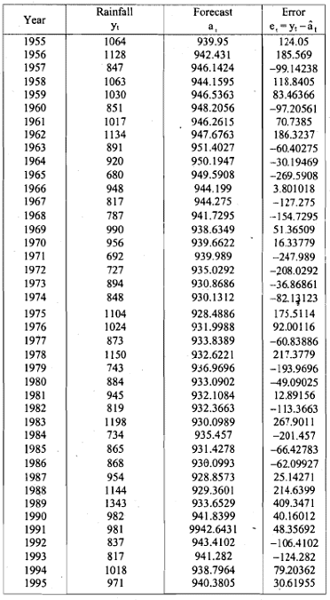
In the table below we have given all the forecasts and errors.
Table: Exponential Smoothing of Rainfall Data
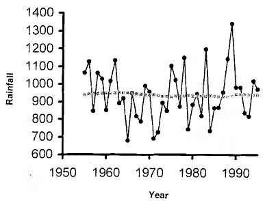
 Now look at the graphs of the time series before and after smoothing, in Fig.. You can see that the peaks are barely there in the graph of the time series after smoothing, which is the dotted curve.
You can also try forecasts with other values of w, and see the curves you get. We still haven't seen what the appropriate choice of w is. For this, we need to consider  that is, the square root of the average error sum of squares. Since this depends on the choice of w, we shall denote it by SE(wj. If we compute this quantity for our rainfall data, we get
  by using the calculations shown in Table. We are now in a position to find out what value of \v is most appropriate for our rainfall data - we should find the value of w for which SE(W) is minimum. How do we find this out? Note that if SE(w) is the minimum for w = α, say, then 4 I (sE(α)2 will be the minimum of all values of (sE- (w))2 calculated for different values of w. So, to find the value of w that gives the least value of SE(w) it is enough to find the error sum of squares, say, (E(w))2 . In Table we give [E(wt)2 for different values of w. Note that SE(w) is small when w = 0.0005 (or w = 0.001). The small value of w indicates that the average level of the time series is not changing much over time.
Using the recursive equation (6) it can be shown that ,

Since (1 - w), (1 - w)2 ., . . are decreasing exponentially, the weightages given to more recent observations is more. So, all the observations are being given weightage here, and the latest observation is being given greatest weightage. In this way, this method is a refinement of the method of moving averages.
- Let us now consider another exponential smoothing forecasting method. This is due to C.C. Holt, suggested by him in 1958.
- Holt’s method: We shall illustrate this procedure with the rice yield data. Suppose that the trend shown by the rice yield data is linear, namely, yt - a + bt + et, where et is the error.
- As before, we shall assume that a and b change gradually over time. Therefore, we denote the values of a and b at time t by at and bt, respectively. As in simple exponential smoothing, at and bt are smoothened using two smoothing constants W1 and W2 (both between 0 and 1). The recursive equations for computing these quantities and the forecasts are given by :
 and the forecast for the immediate future yt+1 s given by

- Here too, we need the initial values a0 and b0. These, together with W1 and w2, should be chosen so that the sum of the squarcs of the forecasting errors ii rninimised. One suggestioil to obtain a0, b0, w1 and w2 is to first obtain ao and bo by fitting a linear regression to one half of the time series data (ao as the intercept and bo as coefficient). Then, using them as initial values, we should obtain the values of wl and w;! which minimise SE, the square root of the average of error sum of squares. Once w and w2 are obtained, then we can change the initial values a. and be to the intercept and coefficient of the regression line titted to the entire time series data. However, there is no guarantee that this would lead to the best choice of ao, bo, wl ahd w2. tn fact, this procedure of obtaining a0, b0, w1 and w2 in our example results in a very large value of SE. A better choice is

- The resulting SE = 133.16. The computations are shown in . Table. The values in the columns have been rounded off to the nearest integer for simplification in calculations.
Table: Holt's Exponential Smoothing of Rice Yield Data
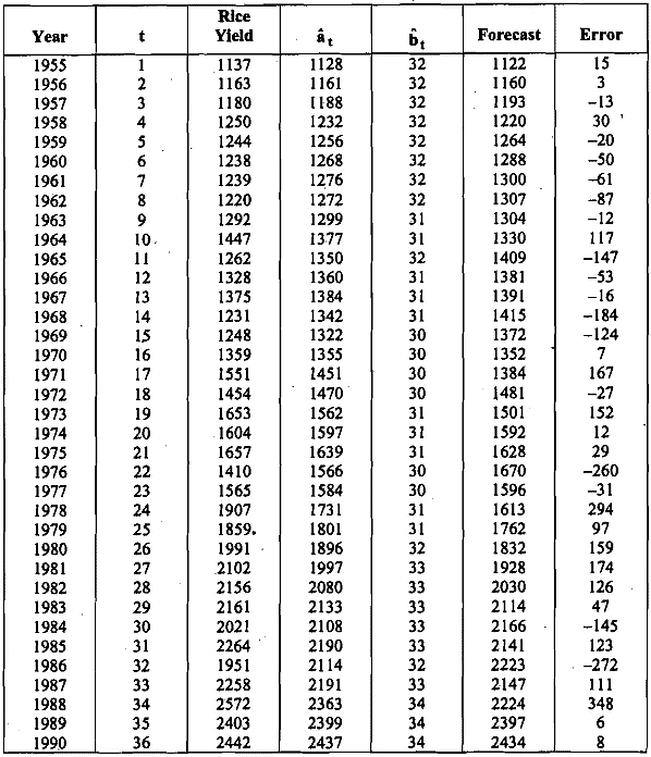 The forecasts and the actual time series values are plotted in Fig.
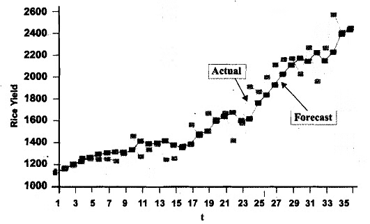
Fig.: Forecast with Holt's model
Now, observe Equation (9), which gives forecasts of the immediate future. Assume that we have got the data only upto 1985, and that we wish to forecast the yields from 1986 to 1990. Note that t = 31 corresponds to year 1985. Equation (9) can now be generalised to make these forecasts as follows :

FAQs on Time series and forecasting - 2 - Management Optional Notes for UPSC
| 1. What is the importance of forecasting models in analyzing long-term trends? |  |
| 2. How do forecasting models help in the context of the UPSC exam? |  |
| 3. What are some commonly used forecasting models for analyzing long-term trends? |  |
| 4. What are the limitations of forecasting models in predicting long-term trends? |  |
| 5. How can UPSC aspirants utilize forecasting models effectively in their preparation? |  |


