Revenue Class 12 Economics
| Table of contents |
|
| Introduction |
|
| Perfect Competition: Defining Features |
|
| Revenue |
|
| Profit Maximisation |
|
| Supply Curve of a Firm |
|
| Determinants of Supply Curve |
|
| Market Supply Curve |
|

Introduction
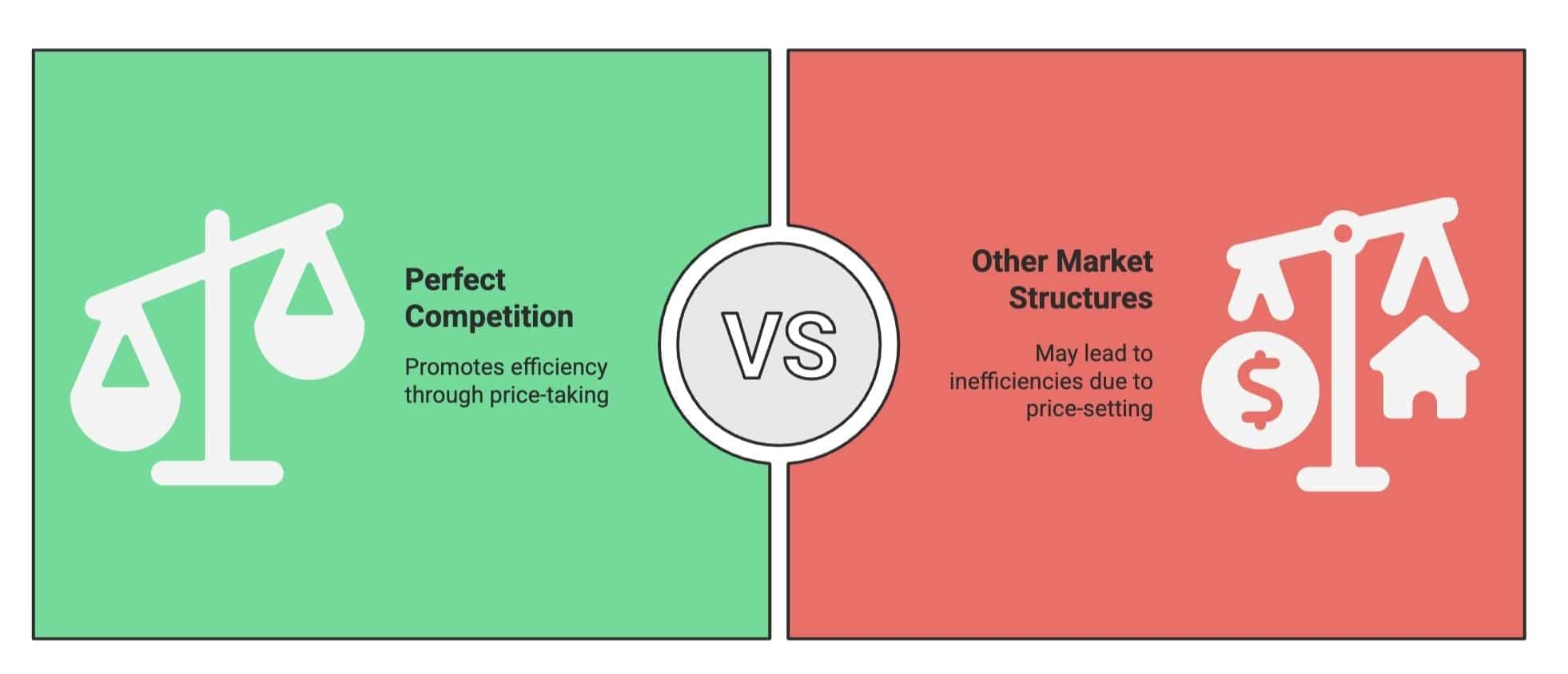
Perfect competition is a market where many buyers and sellers trade identical products, with no one able to set prices. Everyone is a price-taker, accepting the market price. Understanding perfect competition is fundamental in economics as it illustrates how markets can achieve efficiency under ideal conditions and provides a standard for comparing other market structures.
Perfect Competition: Defining Features
A market is a place or system where buyers and sellers interact to exchange goods and services at agreed-upon prices. A perfectly competitive market is a type of market where many buyers and sellers come together to trade a single, identical product. No one—whether a buyer or a seller—has the power to control the price.
Let’s understand the key features that make this market “perfectly competitive”:
1. Many Buyers and Sellers: There are a large number of buyers and sellers in the market. Each one is very small compared to the whole market. So, no single buyer or seller can influence the price.
2. Homogeneous Product (Identical Product): Every seller sells the exact same product. For example, if two farmers are selling wheat, there’s no way to tell the difference between their wheat. This means buyers can buy from any seller and still get the same product.
3. Free Entry and Exit: Firms (sellers) are free to join or leave the market at any time.
- If making profits, new firms can enter easily.
- If facing losses, firms can exit without restrictions.
- This keeps the number of sellers balanced over time.
4. Perfect Information: Everyone in the market—both buyers and sellers—has complete knowledge about prices being charged, quality of the product and other important details. This helps buyers make smart choices and stops sellers from charging unfair prices.

What is Price-Taking?
The most important feature of perfect competition is price-taking.
For Sellers: A firm (seller) cannot choose its own price.
- If it tries to charge more than the market price, buyers will go to other sellers.
- If it charges the same or less, it can sell as much as it wants.
For Buyers: A buyer cannot offer a lower price than the market price.
- If she does, no seller will sell to her.
- If she agrees to pay the market price or more, she can buy as much as she needs.
Why Do Firms and Buyers Accept the Market Price?
Let’s say every firm sells the product at ₹10 (market price). If one firm starts selling at ₹12:
- Buyers will not buy from this firm, because they can get the same product elsewhere for ₹10.
- Since there are many other sellers, buyers can easily switch without any problem.
This is why, in a perfectly competitive market, everyone accepts the market price and no one tries to set their own. That’s what we mean by price-taking behaviour.
Revenue
Revenue is the income a firm earns from selling its goods or services.
Total Revenue (TR)
- The price (p) of the commodity is multiplied by the amount produced and sold to determine revenue (q).
- Total revenue (TR) is defined as
TR = p × q
Total Revenue Curve
- The relationship between the total revenue earned by a firm for selling its output and the quantity of output sold is visually represented by a curve. Let's understand this with the help of an example.
- For a candle manufacturer, the market price per box is Rs 10. TR depends on the quantity sold (Q).
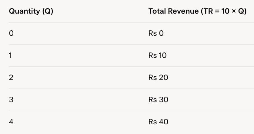
When no boxes are sold, Total Revenue (TR) is zero. Selling one box of candles gives TR = 1 × Rs 10 = Rs 10; selling two boxes gives TR = 2 × Rs 10 = Rs 20, and so forth.
The Total Revenue (TR) Curve illustrates how total revenue varies with the quantity sold. It plots quantity (output) on the X-axis and revenue on the Y-axis, as shown in the figure. Three key points stand out:
- When output is zero, TR is also zero, so the TR curve starts at the origin (point O).
- As output increases, TR rises, and since the price (p) is constant, the equation TR=p×q forms a straight line, making the TR curve a linear, upward-sloping line.
- The slope of the TR curve is determined by the price (p). For one unit of output (horizontal distance Oq1 in the figure), TR is p × 1 = p (vertical height Aq1). Thus, the slope is Aq1/Oq1 = p.

Average Revenue
- The income earned per unit of output is referred to as average revenue.
- In other words, it is the profit earned by the seller on each unit of the commodity sold.
- The average revenue of a company is calculated by dividing total revenue by total output.

Price Line
- The price line and demand curve for an individual firm in a completely competitive market are the same.
- The line denotes that a company's goods and services may be sold at the current price.
- The price line in such a market is a horizontal straight line that depicts that the firm can sell any quantity of a product only at a certain price. If the firm tries to change the price, the overall demand falls to zero, because as there are a large number of small firms, no firm is capable enough to impact the overall price or supply.
- The price line is shown below:

Marginal Revenue
- The revenue generated by selling an additional unit of a commodity is known as marginal revenue.
- When an additional unit of a commodity is sold on the market, it results in a change in overall revenue.
- The following equations can be used to describe the link between market price and marginal revenue:

TR = Total Revenue
MR = Marginal Revenue
Q = Quantity - In a perfectly competitive market, the price equals marginal revenue, according to the preceding equation.
MR = PQn − PQn-1
or
Understanding Marginal Revenue with an Example
Imagine you have a small bakery selling cupcakes.
- When you sell 2 cupcakes, you earn Rs. 30.
- When you sell 3 cupcakes, you earn Rs. 45.
Now, let’s find out how much extra money you made by selling that 1 extra cupcake.
- Change in Total Revenue = Rs. 45 - Rs. 30 = Rs. 15.
- Change in Quantity = 3 - 2 = 1.
So, Marginal Revenue (MR) = 15/1 = Rs. 15.
That means, by selling 1 more cupcake, you earned an extra Rs. 15.
Is Marginal Revenue Always the Same as Price?
Yes! For a bakery in a perfectly competitive market, the Marginal Revenue (MR) is always equal to the market price (p).
The relationship between MR and Price
We can prove that MR = Price (p) under perfect competition:

The relationship between marginal revenue and pricing is depicted graphically as follows:
TR, MR and AR Curves in a perfectly competitive market can be seen in the graph below:

Profit Maximisation
Imagine a toy-making company that produces and sells a certain number of toys. The company's profit (π) is simply the difference between the money it earns from selling toys (Total Revenue, TR) and the money it spends on making them (Total Cost, TC). So,
Profit (π) = TR – TC.
The bigger the gap between TR and TC, the higher the profit. Naturally, the company wants to make this gap as big as possible. But how do they find the perfect number of toys to produce (q0) to get the most profit?
To Maximise Profit, These Conditions Must Be Met:
- Price (p) must equal Marginal Cost (MC): The company makes the most profit when the money earned from selling one more toy is exactly the same as the cost of making that toy.
- Marginal Cost Should Not Decrease at q0: The cost of making each extra toy shouldn’t keep dropping at the profit-maximising point.
- Price Must Cover Costs:
- Short Run: The price should be higher than the Average Variable Cost (AVC).
- Long Run: The price should be higher than the Average Cost (AC).

Condition 1: Maximising Profit by Comparing Revenue and Cost
A company's profit is the difference between the money it earns (Total Revenue) and the money it spends (Total Cost). As the company produces and sells more products, both Total Revenue and Total Cost increase.
Now, here's the key:
- If the extra revenue earned from selling one more unit (Marginal Revenue, MR) is greater than the extra cost of producing that unit (Marginal Cost or MC), then profits will keep increasing.
- But if the MR is less than the MC, the company’s profit decreases.
To make the most profit, the company needs to produce up to the point where Marginal Revenue equals Marginal Cost (MR = MC).
In a perfectly competitive market, MR = Price (P). So, the company will earn the most profit when it produces up to the point where P = MC.
Condition 2: Why Marginal Cost Can't Slope Downward for Maximum Profit
For a firm to achieve the highest profit, the Marginal Cost (MC) curve should not slope downward at the profit-maximising point. But why?
Imagine two output levels: q1 and q4. At both points, the market price is the same as the MC. However, at q1, the MC curve is sloping downward.
Now, look at the outputs slightly to the left of q1. The market price is lower than the MC. According to the profit rule we learned earlier, the company’s profit will actually be higher if it produces slightly less than q1.
Since producing at q1 doesn’t give the highest possible profit, q1 cannot be the profit-maximising output. The MC curve must be flat or upward-sloping at the point where profit is highest.

Condition 3: Price Must Cover Costs to Keep Producing
For a firm to make the most profit, it must consider whether it’s operating in the short run or the long run. Let's understand both of these cases.
Case 1: Short Run (Price ≥ AVC)
In the short run, a company will only keep producing if the market price is at least equal to the Average Variable Cost (AVC).
Why?
If the price is lower than the AVC, the firm is losing more money by producing than it would by simply shutting down. It’s like running a lemonade stand where each glass costs Rs. 5 to make (AVC), but you’re only able to sell them for Rs. 3. You’d be better off not selling at all!

Understanding the Concept with the Figure
Imagine a firm producing at an output level q1, where the market price (p) is lower than the AVC. Here’s what happens:
- Total Revenue (TR) = Price × Quantity = Area of rectangle OpAq1.
- Total Variable Cost (TVC) = AVC × Quantity = Area of rectangle OEBq1.
Now, compare the two areas:
- The firm’s loss at q1 is: TR - TVC - TFC = (OpAq1) - (OEBq1) - TFC.
- Clearly, the revenue OpAq1 is less than the cost OEBq1.
What if the Firm Produces Nothing?
- If output = 0, then TR = 0 and TVC = 0.
- The firm’s loss would only be its Total Fixed Cost (TFC).
Since the loss at q1 is even greater than just TFC, it’s better for the firm to stop production entirely rather than produce at a loss.
In short, if the market price (p) is below the AVC, the firm will choose to produce nothing because it's losing more money by producing than by stopping.
Case 2: Price Must Cover Average Cost in the Long Run
In the long run, a profit-maximising firm will only continue producing if the market price is equal to or above the Average Cost (AC). Let’s break down why.

Imagine a firm producing at an output level q1, where the market price (p) is below the Average Cost (AC). Here’s what happens:
- Total Revenue (TR) = Price × Quantity = Area of rectangle OpAq1.
- Total Cost (TC) = Average Cost × Quantity = Area of rectangle OEBq1.
Since the area representing Total Cost (OEBq1) is larger than the area representing Total Revenue (OpAq1), the firm is incurring a loss at this output level.
What if the Firm Stops Producing?
- In the long run, a firm that stops production altogether has a profit of zero.
- Producing at q1 gives a loss, so the firm would prefer to exit the market completely.
To stay in business, the market price must be at least equal to AC.
The Profit Maximisation Problem: Graphical Representation
Let's understand how a firm maximises its profit through a graphical representation.
Imagine a firm trying to find the best output level where it can make the most profit. Here's how it works:
- The firm produces at output level q0, where the market price (p) equals the Short Run Marginal Cost (SMC).
- The SMC curve slopes upwards at this point, and the market price (p) is higher than the Average Variable Cost (AVC), which meets all three conditions for profit maximization.
- Total Revenue (TR) at q0 = Area of rectangle OpAq0 (Price × Quantity).
- Total Cost (TC) at q0 = Area of rectangle OEBq0 (Short Run Average Cost × Quantity).
- Therefore, the firm's profit is the area of rectangle EpAB.
The key takeaway? When the price is higher than the cost of producing each unit (SMC), the firm makes a profit.
Supply Curve of a Firm
When we talk about a firm’s supply, we’re simply talking about how much of a product a firm is willing to sell at a particular price. But there’s a catch! This supply is based on three things:
- The price of the product
- The technology available
- The prices of factors of production (like labour, raw materials, etc.)
Supply Schedule:
- A supply schedule is a table that shows the amounts sold by a company at various prices while keeping technology and factor prices constant.
Supply Curve:
- The supply curve of a firm depicts the amounts of output that the firm chooses to create in response to varied market price values while maintaining technology and factor prices constant.
Short Run Supply Curve of a Firm
To figure out how a firm decides its supply in the short run, we need to consider two cases:
Case 1: When Market Price is Greater Than or Equal to Minimum AVC
Imagine the market price is p1, which is higher than or at least equal to the minimum Average Variable Cost (AVC). Here’s what happens:
- The firm looks at where the price line (p1) meets the upward-sloping part of the Short Run Marginal Cost (SMC) curve.
- This point of intersection determines the output level, q1.
- Since the price is higher than the AVC, the firm is covering its variable costs and some of its fixed costs, so it continues producing.
In simpler words, as long as the firm can sell its product at a price that covers its cost of making each extra unit (AVC), it’s in business!
Case 2: Price is less than the minimum AVC
- Presume the market cost price is P2, which is lower than the AVC minimum.
- If a profit-maximising firm produces a positive output in the short run, the market cost price, P2, has to be higher than or equal to the AVC at that output level.
- The AVC clearly outperforms P2 in the image.
- To put it another way, the company is unable to generate a profit. As a result, if the market price is P2, the enterprise produces no output.

Combining Case 1 and Case 2
Combining both cases gives us a simple but important conclusion:
- The short-run supply curve of a firm is the upward-sloping part of the SMC curve starting from and above the minimum AVC.
- If the market price is below the minimum AVC, the firm’s supply is zero.
Long-Run Supply Curve of a firm
- When all inputs are variable, the long-run supply is the supply of commodities available.
- The supply curve, in the long run, is always more elastic than the supply curve in the short run.
- In a U-shaped curve, the long-run average cost curve encompasses the short-run average cost curves.
- With the addition of increasing long-run marginal cost curves, the supply curve is upward-sloping.

Case 1: Price greater than or equal to the minimum LRAC
- Presume the market cost price is P1, which is greater than the minimum LRAC. We obtain the output degree Q1 by equating P1 with LRMC on the increasing part of the LRMC curve.
- It's also worth noting that the LRAC in Q1 does not exceed the market cost price, P1.
- As a result, at Q1, all three of the conditions are met. When the market cost price is P1, the firm's supplies are equal to Q1 in the long run.

Case 2: Price less than the minimum LRAC
- Assuming the market cost price is P2, which is lower than the LRAC minimum.
- If a profit-maximising firm produces a positive output over time, the market cost price, P2, must be larger than or equal to the LRAC at that production level.
- In other words, the firm is unable to produce a positive result. As a result, when the market cost price is P2, the firm produces nothing. We reach an important conclusion by combining Cases 1 and 2.
- The long-run supply curve of a business is the increasing section of the LRMC curve from and above the minimum LRAC, as well as the zero production for all-cost prices less than the minimum LRAC.

The Shut Down Point
While deriving the supply curve, we noted that a firm continues to produce in the short run as long as the price is at least equal to the minimum of the Average Variable Cost (AVC). So, as we move down along the supply curve, the last price-output combination where the firm produces positive output occurs where the Short Run Marginal Cost (SMC) curve intersects the AVC curve at its minimum point.
If the price drops below this point, the firm ceases production. This point is known as the short-run shutdown point of the firm. In the long run, however, the shutdown point is determined by the minimum of the Long Run Average Cost (LRAC) curve.
The Normal Profit and Break-even Point
The normal profit is the minimum level of profit needed for a firm to continue operating in its current business. If a firm fails to earn this amount, it won't stay in business. Normal profit is considered a part of the firm’s total costs and can be seen as the opportunity cost of entrepreneurship.
When a firm earns profit above normal profit, it is called super-normal profit.
- In the long run, a firm will not operate if it earns less than the normal profit.
- In the short run, however, the firm may continue producing even if profits are below normal profit.
The point on the supply curve where a firm earns only normal profit is called the break-even point. This occurs where the supply curve intersects the LRAC curve at its minimum point (or the SAC curve in the short run).
Opportunity Cost
In economics, the term opportunity cost refers to the benefit that is given up when choosing one activity over the next best alternative. It represents the potential gain lost from the second-best option that is not chosen.
For example, imagine you have Rs 1,000 and decide to invest it in your family business. What is the opportunity cost of this decision?
- If you keep the money at home, it earns zero return.
- If you deposit it in bank-1, you earn an interest of 10%.
- If you deposit it in bank-2, you earn an interest of 5%.
The best alternative to investing in your family business is depositing the money in bank-1, where you would earn the highest interest of 10%. However, by investing the money in your family business, you lose the opportunity to earn that interest.
Therefore, the opportunity cost of investing the money in your family business is the interest you would have earned from bank-1 (10%).
Determinants of Supply Curve
In the previous section, we established that a firm’s supply curve is a segment of its marginal cost (MC) curve. Therefore, any factor that influences the MC curve also affects the firm's supply curve.
In this section, we will discuss two important factors that impact the supply curve:
Technological Progress
When a firm uses two factors of production, like capital and labour, to produce a good, a technological improvement (such as an organisational innovation) can enhance productivity. This means:
- More output is produced with the same amount of capital and labour.
- Alternatively, the firm can produce the same amount of output using fewer inputs.
This improvement lowers the firm's marginal cost (MC) at any given level of output, causing a rightward or downward shift of the MC curve.
Since a firm's supply curve is part of the MC curve, technological progress shifts the supply curve to the right.
As a result, at any market price, the firm supplies more units of output.
Input Prices
The prices of inputs (such as wages for labour) also affect a firm's supply curve.
- If the price of an input increases (e.g., higher wage rates), the cost of production rises.
- This increase in cost leads to a rise in both the average cost (AC) and marginal cost (MC) at any output level.
The MC curve shifts leftward or upward, causing the firm’s supply curve to shift to the left.
As a result, at any market price, the firm supplies fewer units of output.
Impact of a Unit Tax on Supply
A unit tax is a tax imposed by the government per unit of output sold. For example, if the unit tax is Rs 2, then a firm producing and selling 10 units of a good must pay a total tax of 10 × Rs 2 = Rs 20.

Effect on the Long-Run Supply Curve
When a unit tax is imposed, it increases both the long-run average cost (LRAC) and long-run marginal cost (LRMC) by the amount of the tax (Rs t) at any level of output.
- Before Tax: The firm's LRMC and LRAC are represented by LRMC0 and LRAC0.
- After Tax: With the imposition of the unit tax, the curves shift upward to LRMC1 and LRAC1.
Since the long run supply curve of a firm is the rising part of the LRMC curve above the minimum LRAC, the unit tax shifts the supply curve to the left.
- At any given market price, the firm now supplies fewer units of output.
Market Supply Curve
The market supply curve shows the total output produced by all firms in a market at different market prices.
How is the Market Supply Curve Derived?
Consider a market with n firms: firm 1, firm 2, firm 3, and so on. If the market price is fixed at p, then the total market supply at that price is calculated by adding up the supply of each firm at that price.
Market Supply = [Supply of firm 1 at price p] + [Supply of firm 2 at price p] + ... + [Supply of firm n at price p].
Geometric Representation (Two Firms Example)
Suppose there are two firms with different cost structures:
- Firm 1 will produce only if the market price is greater than or equal to p1.
- Firm 2 will produce only if the market price is greater than or equal to p2 (where p2 > p1).

How the Market Supply Curve is Constructed:
When the market price is below p1:
- Neither firm produces anything.
- Market supply is zero.
When the market price is between p1 and p2:
- Only Firm 1 produces.
- The market supply curve coincides with the supply curve of Firm 1.
When the market price is above p2:
- Both Firm 1 and Firm 2 produce.
- The total supply is the sum of the outputs of Firm 1 and Firm 2 at that price.
- The market supply curve is obtained by horizontally adding the supply curves of the two firms.
Understanding Market Supply Curve with a Numerical Example
The market supply curve we derived before assumed a fixed number of firms. When the number of firms changes, the market supply curve shifts:
- If the number of firms increases, the market supply curve shifts to the right.
- If the number of firms decreases, the market supply curve shifts to the left.
Now, let’s look at a numerical example involving two firms.
Supply Curves of the Firms
1. Firm 1's Supply Curve (S1(p))
When p < 10, the firm produces 0 units.
When p ≥ 10, the output produced is (p - 10).
So,
S1(p) = 0 if p < 10.
S1(p) = p - 10 if p ≥ 10.
2. Firm 2's Supply Curve (S2(p))
When p < 15, the firm produces 0 units.
When p ≥ 15, the output produced is (p - 15).
So,
S2(p) = 0 if p < 15.
S2(p) = p - 15 if p ≥ 15.
3. Market Supply Curve (Sm(p))
The market supply curve is the sum of the individual supply curves, i.e.,

Now, let’s break down the calculation:
- When p < 10: Both firms produce 0 units.

When 10 ≤ p < 15:
- Only Firm 1 produces.

When p ≥ 15:
- Both firms produce.

The market supply curve can be summarised as:

Price Elasticity of Supply
- The price elasticity of supply is a measurement of how sensitive a given good's quantity is to a change in price.
Measurement of Price Elasticity of Supply:
- Price elasticity of supply curve,

WhereΔQ = change in the quantity of the good supplied to the market
ΔP = change in the price of the good
Extreme Cases of Price Elasticity of Supply:
- Perfect elasticity supply (es = ∞): The extreme case of perfect elasticity is when the demanded quantity (Qd) or the supplied quantity (Qs) changes by an enormous amount in response to any change in price. The supply and demand curves are both horizontal in both instances. Ï
- Perfect inelasticity supply (es = 0): If a given quantity of a service or commodity can be supplied at any price, it has a perfectly inelastic supply. The supply elasticity of such a service or commodity is zero. A straight line parallel to the Y-axis is a perfectly inelastic supply curve. This illustrates how supply remains constant regardless of price.

Equilibrium Price:
- It is the point at which the supply of commodities equals the demand.
- When a major index undergoes a period of consolidation or sideways motion, the forces of supply and demand are considered to be relatively equal, and the market is said to be in a condition of equilibrium.
Equilibrium Quantity:
- When there is no scarcity or excess of a product on the market, it is said to be in equilibrium quantity.
- When supply and demand meet, the quantity of an item that customers want to buy equals the quantity that producers are willing to produce.
Application of Demand Supply:
- Maximum Price Ceiling: This refers to the lowest price that sellers are permitted to charge in comparison to the equilibrium market price. When the demand for necessary products exceeds the supply, the government imposes a ceiling. That is, when there are shortages among consumers and the equilibrium price is excessively high. It is done by the government in the benefit of consumers. Rationing and dual marketing may be used to meet excess demand.

- Minimum Price Ceiling: This means that producers are not allowed to sell their goods below the price set by the government. If the government determines that the equilibrium price is too low for the produce it sets a price ceiling higher than the equilibrium price to protect producers from potential losses. The price is also known as the minimum support price or the floor price. In most cases, the government purchases the extra supply at this price.

Effect of Technological Advancement on Supply Curve
- The marginal cost of production is reduced as technology advances. With the help of accessible factors of production, producers can generate significantly more goods and services. The supply curve is anticipated to shift rightward and the marginal cost curve is downward because of this circumstance.
- Supply and technical growth have a beneficial relationship.
- Technological advancements frequently result in lower production costs, allowing manufacturers to produce and sell more goods and services at the same price.
- As a result, technological advancement is expected to boost supply, leading the supply curve to shift to the right.

|
59 videos|222 docs|43 tests
|
FAQs on Revenue Class 12 Economics
| 1. What is the market price line in perfect competition? |  |
| 2. How do firms achieve profit maximization in perfect competition? | |
| 3. What is the significance of the profit equilibrium point for firms in a perfectly competitive market? | |
| 4. Can firms in perfect competition earn long-term profits? | |
| 5. How does the concept of revenue relate to the market price line in perfect competition? | |


video lectures
,Viva Questions
,Summary
,ppt
,Previous Year Questions with Solutions
,Objective type Questions
,Free
,Exam
,shortcuts and tricks
,MCQs
,Revenue Class 12 Economics
,Extra Questions
,Revenue Class 12 Economics
,Sample Paper
,past year papers
,Semester Notes
,study material
,Important questions
,Revenue Class 12 Economics
,practice quizzes
,mock tests for examination
;


Chapter Notes - The Theory of the Firm under Perfect Competition Free PDF Download
Importance of Chapter Notes - The Theory of the Firm under Perfect Competition
Chapter Notes - The Theory of the Firm under Perfect Competition
Chapter Notes - The Theory of the Firm under Perfect Competition Commerce Questions
Study Chapter Notes - The Theory of the Firm under Perfect Competition on the App
|
© EduRev
|
Education Revolution
|


|


