Sampling - Sampling & Reconstruction

Sampling
What is sampling?
Sampling is a method of representing a continuous signal by a set of values taken at selected instants of the independent variable. In other words, instead of specifying the dependent variable for every possible value of the independent variable, we specify its values at appropriately chosen points and, together with any available apriori information about the signal, reconstruct the original signal.
Illustrative examples
Consider a continuous-time signal x(t) whose independent variable is time t and dependent variable is the signal amplitude.
If x(t) is a pure sinusoid with amplitude, angular frequency and phase constant, then knowledge of these three parameters suffices to determine x(t) for all t. Thus three independent pieces of information (the parameters) replace the need to know the signal value at every instant.
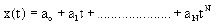
Consider another signal which is a polynomial in t of degree N. Such a signal is completely determined by its coefficients a0, a1, ..., aN. Therefore, knowing the coefficient values is equivalent to knowing the signal at all times.
A common approach to economical signal representation
The usual approach in sampling and reconstruction is to record the values of the signal at suitably chosen values of the independent variable, and use those samples together with the apriori information about the signal class to reconstruct the signal exactly.
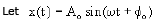
For example, if we know in advance that x(t) is a sinusoid of the form A0 cos(ω0t + φ), then the three parameters A0, ω0 and φ completely characterise the signal. If we measure the signal at three distinct times t1, t2, t3, we obtain three independent equations in these three unknowns and can solve for the parameters.
When describing the sinusoid parameters we may write the phase constant as φ (

For suitably chosen t1, t2, t3 we obtain three independent measurements and therefore three equations:
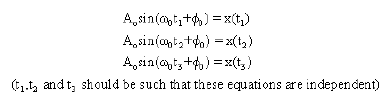
From the observed values x(t1), x(t2) and x(t3) at those instants, the parameters A0, ω0 and φ can be determined. The numerical solution depends on the chosen times and on the measured values.
Consider another example. Let x(t) be a polynomial of order N,
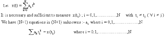
Written as a system of linear equations in the coefficients, the left-hand matrix is a Vandermonde matrix formed from the chosen sample instants. The system can be solved (and the coefficients determined uniquely) so long as the determinant of this matrix is non-zero.

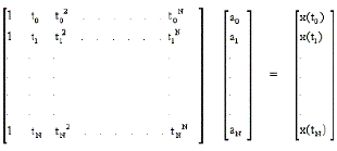
Thus, given the apriori information (for example that the signal is a polynomial of degree at most N), the entire signal can be reconstructed from N + 1 samples taken at appropriate distinct points.
Apriori information and its role
Apriori information is any knowledge about the class of signals to which the unknown signal belongs. Examples include the facts that a signal is sinusoidal, is a polynomial of a given degree, is band-limited, or is continuous. The more restrictive the apriori information, the fewer samples are needed for exact reconstruction.
Knowing only that a signal is continuous is much weaker information than knowing it is a sinusoid. The set of all sine functions is much smaller than the set of all continuous functions; hence the sinusoidal assumption provides more apriori information and allows a much more compact description.
Formal notions: sample sequence and sampling interval
When we sample a continuous-time signal x(t) at uniform intervals of time Ts, we obtain a discrete-time sequence
x[n] = x(n Ts), n ∈ ℤ.
The sampling frequency is fs = 1 / Ts and the angular sampling frequency is 2πfs. The choice of Ts (or fs) is central to the ability to reconstruct the original signal without loss.
Band-limited signals, sampling theorem and aliasing (preview)
A very important class of apriori information is that the signal is band-limited: its Fourier transform is zero outside a finite frequency interval [-B, B]. For this class there is a precise condition that guarantees exact reconstruction from uniform samples. This condition and the reconstruction method are central results in sampling theory and will be treated in detail later.
Informally, the condition requires the sampling frequency to be greater than twice the highest frequency present in the signal (the Nyquist rate), and exact reconstruction is achieved by ideal low-pass filtering of the sampled signal (sinc interpolation). If sampling is done too slowly, different frequency components overlap in the sampled spectrum; this phenomenon is called aliasing and leads to irreversible distortion in reconstruction.
Types of sampling and practical considerations
- Uniform sampling: Samples are taken at equal time intervals Ts. This is the standard case used in most theory and practice and leads to well-developed reconstruction methods.
- Non-uniform sampling: Samples taken at unequal instants. Reconstruction is possible under suitable conditions and using more general methods (for example, solving linear systems or using specialised interpolation), often requiring more samples or heavier computation.
- Ideal sampling (impulse sampling): The continuous-time sampled signal is modelled as a train of weighted impulses: xs(t) = ∑ x(nTs) δ(t - nTs). This ideal model is useful for theoretical analysis of the sampled spectrum and reconstruction.
- Practical issues: Anti-aliasing filters are applied before sampling to limit the signal bandwidth and prevent aliasing. Quantisation of sample amplitudes (in analogue-to-digital conversion) introduces additional approximation error, which is addressed separately.
Reconstruction idea
The general reconstruction idea is to convert the set of samples back into a continuous-time signal using an appropriate interpolator that uses the apriori information. For band-limited signals, the ideal reconstructor is an interpolation by shifted sinc functions weighted by the sample values. For polynomial signals or signals from other finite-dimensional signal classes, reconstruction reduces to solving a finite linear system (for example, via inversion of a Vandermonde matrix when sample times are distinct).
Conclusion
From this chapter you should take away the following points:
- Sampling is a method of using apriori information about a signal to represent it economically by a finite or countable set of values.
- The most common approach in sampling and reconstruction is to record the signal values at selected points on the time axis and use those samples together with apriori information to reconstruct the signal.
- The main challenge in sampling and reconstruction is to make the best use of available apriori information so that the signal can be represented and recovered most economically.
- For special classes of signals (for example band-limited signals) there are precise sampling criteria and reconstruction formulae; these will be studied next, together with the concepts of the Nyquist rate, aliasing and practical reconstruction methods.
FAQs on Sampling - Sampling & Reconstruction
| 1. What is sampling and reconstruction? |  |
| 2. Why is sampling important in signal processing? | |
| 3. What is the Nyquist-Shannon sampling theorem? | |
| 4. What are the common techniques used for signal reconstruction? | |
| 5. Can sampling and reconstruction introduce errors in the signal? | |


 | Explore Courses for Electrical Engineering (EE) exam |
 | Get EduRev Notes directly in your Google search |