Land Leveling Methods, Irrigation Engineering | Irrigation Engineering Notes - Agricultural Engineering PDF Download

A precise land leveling improves irrigation and energy efficiency. This also reduces labor requirement for water application. A properly leveled land can be properly irrigated and excess water can be drained out. However, major topographical changes in the process of land leveling may reduce crop production in the cut areas or additional soils may have to be added in cut areas for improving soil fertility. Further farm machineries movement compact soil and disturb soil pores and thereby reduces water movement through side. Hence it is essential to estimate locations and volumes of cuts and fills, maintain proper cut-fill ratio by minimally affecting the crop production and at the same time involving the less cost for land leveling. Hence for land leveling design should be done properly. There are several methods for land leveling design. These methods are: Plane method, Profile method, Plan inspection method and Contour adjustment methods. The procedures adopted to use these methods are briefly presented in this lesson.

18.1 Plane Method

The plane method is the most commonly used method of land levelling design. This method is feasible whenever it is required to grade the field to a true plane. The procedure involves first determining the centroid of the field as per the procedure explained in section 17.3 of lesson 17 and then determining the average elevation of the field. This is obtained by adding the elevations of all grid points in the field and dividing the sum of elevations by number of grid points. Any plane passing through the centroid at average elevation will produce equal volume of cut and fill. Based on the longitudinal down field grade and cross field grade required for the field, the elevation of each grid points are computed from estimated centroid. The following example illustrates the method to estimate average elevation and elevation at different grid points for a desired slope.

Example 18.1: The elevations of grid points selected at 25 m interval are determined from a topographic survey for land leveling programme. The elevations of points are as given below in the table.

The field is to have downfield slope of 0.2%. Determine: i) elevation of centroid of the field, and ii) formation levels at grid points and amount of cut and fill at each grid point.

Solution:

Total number of stations = 20                         

Sum of the elevations of the 20 stations = 1947.92 m

Elevation of the centroid  m

The field is to be given 0.2% slope. At 50 m from the North South line passing through centroid, the elevation of this point is 0.1 m below the centroid, or 97.296 m.

The formation of grid levels at each point are estimated as given in this table

Cuts and Fills

Cut and fill are computed by subtracting the original elevation of the point from the formation level at the grid point. At station A1, the cut/fill is 97.296 – 97.30 = (-) 0.004. The results of cut / fill are given in following table.

(+ Sign indicates fill and – sign indicates cut)

Σ cut = Σ fill = 6.426 m

Computation of Slopes of Plane of Best Fit

The computation of slopes of plane of best fit is given by

E = a + S_x X + S_y Y                                            (18.1)

where,                    

E = elevation at any point (L)

a = elevation at the origin (L)

S_x and S_y = slope in the x and y directions, respectively (L/L)

X any Y = distance from the origin (L)

The slope of any line in X or Y direction is determined by the statistical least – square procedure, (Schwab et al., 1993). The least –squares plane by definition is that which gives the smallest sum of all the squared differences in elevation between the grid points and the plane. It is called the plane of best fit. These slopes can be computed from two simultaneous equations stated below

(ƩX² – n X²_c)S_x + [Ʃ (X_Y) – nX_CY_C ]S_y = Ʃ (X_E) – nX_cE_C         (18.2)

(ƩY² – nY²_c)S_y+ [Ʃ (X_Y) – nX_CY_C ]S_x = Ʃ (Y_E) – nY_c E_C            (18.3)

where  

n = total number of grid points

X_C = X distance to the centroid

Y_c = Y distance to the centroid

E_c = elevation of the centroid (average elevation of all points).

For rectangular fields the terms involving XY become zero and

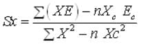(18.4)

The slope S_y can be obtained from Eq. (18.4) by substituting Y for X. Although Eq. (18.4) is valid only for rectangular fields, a satisfactory solution can often be obtained by taking one or more arbitrarily selected rectangular areas within the field and extending the slopes of the plane to the remaining areas.

Average elevation of the field is determined by adding the elevations of all the grids and dividing the sum by number of points.

Example 18.2: Establish the equation for determining the elevation at any point using plane of best fit approach for the field shown in Fig. 18.1.(Elevations of different grids of field are in meter)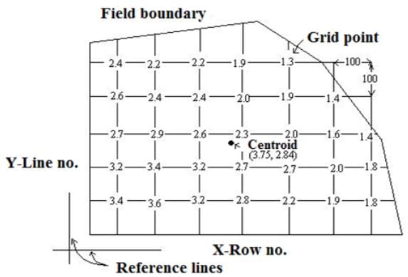

Solution:
The plane of best fit approach uses following equations for determination of slopes in X and Y direction. The following table illustrates the computation procedure for determining plane of best fit.

In X- direction,

(i) Total no. of stakes = 32

(ii) Product = 120     

(iii) Average

In Y- direction,  

(i) Total no. of stakes = 32

(ii) Sum of product is = 91

(iii) Average  

Hence co-ordinates of centroid = (3.75, 3.84)

No. of stakes (n) = 32, X_C  = 3.75,Y_C  = 2.84

E_c= (3.4 + 3.2+ 2.7 +…. + 1.8 +1.4) / 3² = 2.37 m

∑X²  = 1² + 1² + 1² + 1² + 1² + 2² +…. + 6² + 7² + 7² + 7² = 566

nX_C² = 3² × 3.75² = 450

nY_C² = 3² × 2.84² = 258.1

∑ (Y_E) = 204.2

nY_c E_c = 32 × 2.84 × 2.37 = 215.4

∑ (X_Y) = (1×1) + (1×2) + (1×3) +….(7×1) + (7×2) + (7×3) = 327

nX_c Y_c = 32 × 3.75 × 2.84 = 340.8 

∑ (X_E) = 255.8

nX_c E_c = 32 × 3.75 × 2.37 = 284.4

Equation (18.2) is replaced here

(ƩX² – n X²_c)S_x + [Ʃ (X_Y) – nX_CY_C ]S_y = Ʃ (X_E) – nX_cE_C                              

or, (566 – 450) S_x + (327– 340.8) S_y = 255.8  –284.4       (18.5)

Equation (18.3) is reproduced

(ƩY² – nY²_c)S_y+ [Ʃ (X_Y) – nX_CY_C ]S_x = Ʃ (YE) – nY_c E_C           

or, (319 – 258.1) S_y+ (327 – 340.8) S_x = 204.2 – 215.4         (18.6) 

From Eq. (18.6)

60.9 S_y – 13.8 S_x = –11.2             (18.7)

From Eq. (18.5)

13.8 S_y + 116 S_x = –28.6          (18.8)

Eq. 18.7 ´ 13.8 ⇒    840.42 S_y – 190.44 S_x = – 165.6    (18.9)                                

Eq. 18.8 ´ 60.9 ⇒   –840.42 S_y + 7064.4 S_x = –1741.74      (18.10)

From Eq. 18.9 and Eq. 18.10

6873.96 S_x = –1896.3

or,    S_x= –0.276 /100 m

From Equation (18.7)

60.9 S_y – 13.8 × (–0.276) = –11.2

or,     S_y = –0.246 /100 m

Since the plane of best fit must pass through the centroid, substituting the above values in Eq. (18.1).

E = a + S_xX + S_yY                                                             (18.12)

or,               2.37 = a +  ((–0.276 ) × 3.75)  +  ((–0.246) × 2.84)

          or,               a = 4.103 m

The elevation of the origin as 4.103 m

Hence elevation at any point in the field is given by E = 4.103 – 0.276 X – 0.246Y

18.2 Profile Method
The profile method of land levelling design consists of plotting the profiles of the grid lines and then laying the desired grade on the profiles. With this method, ground profiles are plotted and a grade is established that will provide an appropriate balance between cuts and fills as well as reduce haul distances to a reasonable limit. It is usually well adopted to leveling design of very flat land with undulating topography on which it is desired to develop a fairly uniform surface relief. Using profile method the designer works with profiles of the grid lines rather with elevations. The profiles are normally plotted in one direction with the individual profiles located on the paper so that the datum line for each profile is in the correct position with adjacent profiles. Profiles may be plotted across the slope or down the slope. Trial grade lines are plotted on each profiles based on the design criteria. The balance between cuts and fill is approximated by eye and comparing the areas between the plotted profiles and the trial grade line. Usually several trials are necessary before a satisfactory set of grade lines are attained. The volume of cut and fill is computed and further adjustment of the grade lines is done to obtain desired cut-fill ratio for the field.

18.3 Plan Inspection Method
The plan inspection method is a rapid method. Although this method does not ensure minimum cuts and fills or the shortest length of haul, however it gives quick estimate. This method is adapted to moderate flat land slopes. A proposed ground surface map is overlaid on the original contour map. Hence it involves contour adjustment using procedure. New contour lines are drawn using uniform slope and spacing between them.

18.4 Contour Adjustment Method
A balance between the cut and fill can be approximated by maintaining the proposed contour in an average position with reference to the original contour at the same elevation. Sum of the design cut and fills from the stake points are compared with total and then readjusted to obtain design levels. Contour adjustment method is adapted to smoothening of steep lands that are to be irrigated. This method demands considerable judgment on the part of designer to keep the earthwork and haul to a minimum. The design grade elevations are determined after a careful study of the topography. It involves trial and error method considering down grade and cross slope limitations.