Block Diagram: Reduction Rules (Detailed Notes) | Control Systems - Electrical Engineering (EE) PDF Download

Block Diagram in Control Systems
Any system can be described by a set of differential equations, or it can be represented by the schematic diagram that contains all the components and their connections. However, these methods do not work for complicated systems.
The Block diagram representation is a combination of these two methods. A block diagram is a representation of a system using blocks.
For representing any system using block diagram, it is necessary to find the transfer function of the system which is the ratio of Laplace of output to Laplace of input.
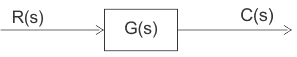
Where
R(s) = Input
C(s) = output
G(s) = transfer function
Then, the system can be represented as
C(s) = R(s).G(s)
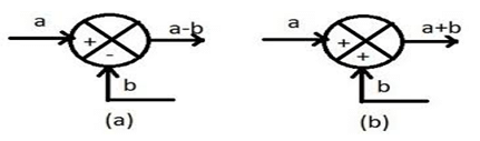
Summing Point: When we want to apply a different input signal to the same block then the resultant input signal is the summation of all the inputs. The summation of an input signal is represented by a crossed circle called summing point which is shown in the figure below.
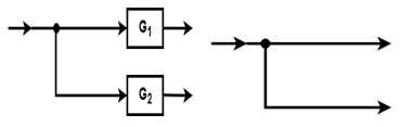
Take off Point: When there is more than one block, and we want to apply the same input to all the blocks, we use a take-off point. By the use of a take-off point, the same input propagates to all the blocks without affecting its value. Representation of same input to more than one block is shown in the below diagram.
How to draw the block Diagram
Consider a simple R-L circuit
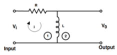
Apply KVL
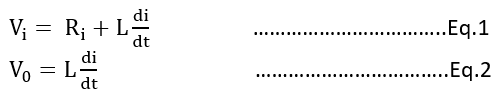
Now taking laplace transform of Eq.1 and Eq.2 with initial condition zero
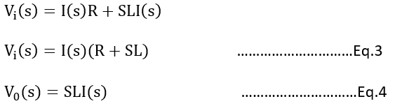
From eq. 3 and eq. 4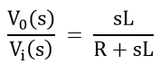 From fig:
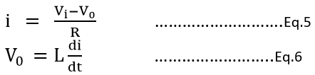 Now taking laplace transform of Eq.5, and Eq.6
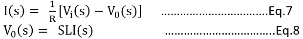
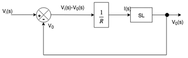
For the right-hand side of eq.5, we will use a summing point.
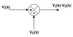
Here the output of summing point is given to the block, and the output of the block is I(s)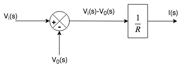
Now the output I(s) is given to another block containing element SL and the output of this block is V0.
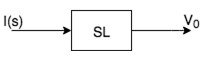
By combining the above two figures, we get the required block diagram
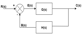
Closed loop control system
A system in which a feedback path is there is called a closed-loop control system. In this system, the output is feedback into the error detector and then it is compared with the input signal. The feedback signal can be negative or positive.
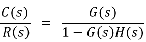
For positive feedback
And for negative feedback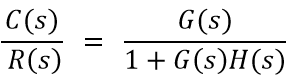
Block diagram reduction rules
Rule No. 1 Blocks in Cascade
When two or more blocks are connected in series, then the resultant block is the product of the individual blocks.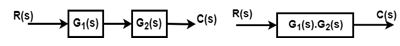 Rule No. 2 Blocks in parallel
When two or more blocks are connected in parallel, then the resultant block is the sum of the individual blocks.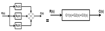 Rule No. 3 Moving a take-off point ahead of a block
When the take-off point is moved ahead of a block (before the block), then the same transfer function is introduced in the take-off point branch.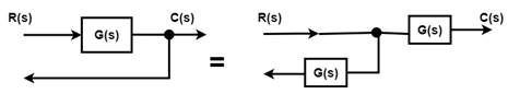 Rule No. 4 Moving the take-off point after the block
When the take-off point is moved after the block, then a block with reciprocal of a transfer function is introduced in the take-off point branch.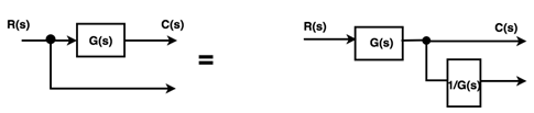 Rule No. 5 Moving a summing point beyond the block
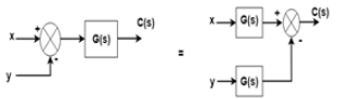
Rule No.6 Moving a summing point ahead of a block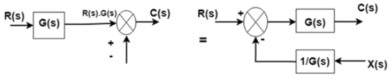 Rule No.7 Interchanging two summing points
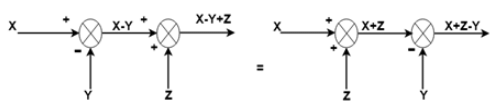
Rule No.8 Moving a take-off point beyond a summing point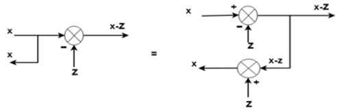 Rule No.9 Moving a take-off point ahead of a summing point
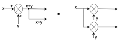
Rule No.10 Eliminating a forward loop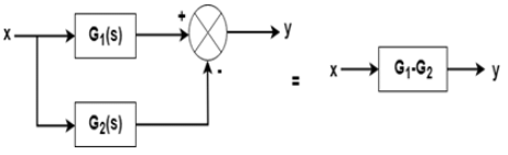
Example
Find the transfer function of the following by block reduction technique.
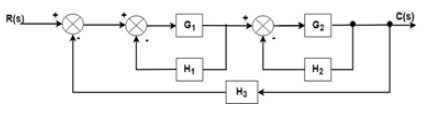
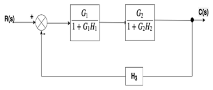
Step 1: There are two internal closed loops. Firstly, we will remove this loop.
Step 2: When the two blocks are in a cascade or series we will use rule no.1.
Step 3: Now we will solve this loop.
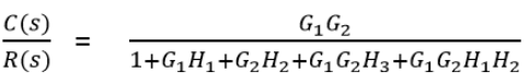
Step 4:
|
53 videos|107 docs|40 tests
|
FAQs on Block Diagram: Reduction Rules (Detailed Notes) - Control Systems - Electrical Engineering (EE)
| 1. What is a block diagram in control systems? |  |
| 2. What are reduction rules in block diagrams? | |
| 3. How do reduction rules help in analyzing control systems? | |
| 4. What are some common reduction rules used in block diagrams? | |
| 5. How do reduction rules help in designing control systems? | |


Semester Notes
,Block Diagram: Reduction Rules (Detailed Notes) | Control Systems - Electrical Engineering (EE)
,Previous Year Questions with Solutions
,ppt
,Viva Questions
,Sample Paper
,Block Diagram: Reduction Rules (Detailed Notes) | Control Systems - Electrical Engineering (EE)
,Block Diagram: Reduction Rules (Detailed Notes) | Control Systems - Electrical Engineering (EE)
,mock tests for examination
,practice quizzes
,Important questions
,study material
,Extra Questions
,Free
,MCQs
,Summary
,Exam
,shortcuts and tricks
,past year papers
,Objective type Questions
,video lectures
;


Block Diagram: Reduction Rules (Detailed Notes) Free PDF Download
Importance of Block Diagram: Reduction Rules (Detailed Notes)
Block Diagram: Reduction Rules (Detailed Notes)
Block Diagram: Reduction Rules (Detailed Notes) Electrical Engineering (EE) Questions
Study Block Diagram: Reduction Rules (Detailed Notes) on the App
|
© EduRev
|
Education Revolution
|


|


