Basic Concepts of Frequency Response | Control Systems - Electrical Engineering (EE) PDF Download

Introduction

• The frequency of the input signal is varied over a specific range, and the system's output is studied. The change in the system's output response with respect to the varied input is known as the system's frequency response.
  
• The frequency response is represented as T(JW), and it comprises of phase function and the magnitude function. They are also known as the system's frequency response, which can be evaluated both for the open-loop and closed-loop systems.
• The open-loop transfer function is given by:
  G(s) = G(jw)
• Where, s = jw
  |G(s)| or |G(jw)|represents the magnitude of the transfer function.
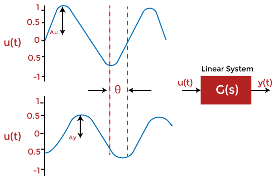
  ∠G(jw) represents the phase of the transfer function.
• Here, we will consider the response of the system with the input at different frequencies. The frequency response is a steady state response of the system to a sinusoidal input signal.
• For example, if a system has sinusoidal input, the output will also be sinusoidal. The changes can occur in the magnitude and the phase shift.
  Let G(s) = 1/(Ts + 1)
• It is the transfer function in the time-constant form. We are assuming all the parameters in the steady state.
  G(jw) = 1/(Tjw + 1)
• Let the input be Asin(wt).
  |G(jw)| = K/(1 + w²T²)^1/2
• It represents the magnitude.
• The angle G(s) is given by:
  tan^-1(Tw)
• The above analysis tells that the steady state output (Css) when the input was Asinwt is given by:
  Css(t) = A.K.sin(wt - tan^-1(Tw))/(1 + w²T²)^1/2

Sinusoidal transfer function

• If the input of the control system is sinusoidal, it is said to be sinusoidal input. Similarly, the system's response when the input is in the form of sinusoidal input is known as a sinusoidal response.
• The sinusoidal transfer function is defined as the ratio of the response of the system to the sinusoidal input, which is given by:
  Sinusoidal transfer function = Response/ sinusoidal input
  It is denoted by T(jw).
  If the sinusoidal transfer function is represented in the frequency domain, it is known as the frequency domain transfer function.

Advantages of frequency response

The advantages of the frequency response method are as follows:

• It includes simple calculations.
• The frequency response method is easy to implement in the designs of the control system. It also helps us to find the stability of the system.
• It provides the stability analysis of the system without the need for any complex and time-consuming processes.
• The frequency response and the step response of the system are closely related. One known parameter gives us the idea of the other parameter.
• We can obtain the frequency response of the given control system without the knowledge of the transfer function.
• The stability analysis of the system can be performed even if it incorporates moderate degree of non-linearity.
• We can also apply the frequency response on the system that has irrational transfer function. For example, e-2Ts.
• It involves simple and inexpensive apparatus.
• In case of the complex cases of the control system, it is better to use the Nyquist plot technique. It is the only method to analyze the stability in such conditions.
• The effect of the noise disturbance can be easily analyzed.
• The adjustment and performance of the closed loop system using the frequency response is easy as compared to the time domain.

Disadvantages of frequency response

The disadvantages of the frequency response method are as follows:

• The frequency response method works better with the linear system. The result in the cases of non-linear systems or the system with moderate non-linearity does not show the exact results. Hence, it is generally applied only to linear systems.
• The practical method to obtain the frequency response is time-consuming.
• There is a relation between the frequency response and the step response, but it is not exact as expected. But, the exact relation is possible if we use the Fourier transformation to describe it, which is difficult to apply due to complex calculations.

Frequency response plot

We can perform the frequency response analysis in the graphical form or the analytical form. The various graphical techniques available for the frequency response analysis are as follows: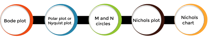

Let's discuss a short description about all the above listed plots.

• Bode plot: It is a frequency response plot that contains two graphs, magnitude and phase. The first plot is the magnitude plot of sinusoidal transfer function versus log w. The other graph represents the phase angle, and it is drawn both for the open-loop and closed-loop system.
• Polar plot or Nyquist plot: It is the plot of the magnitude of the given transfer function to its phase angle on the polar coordinates. The frequency in the polar plot is varied from zero to infinity. The polar plot is drawn on the polar sheet, which is the form of graph. The graph consists of concentric circles and radial lines. The extension of polar plot is known as Nyquist plot. The frequency in the case of Nyquist plot varies from -infinity to infinity.
• M and N circles: It is used to obtain the values of the closed-loop function but from the Nyquist plot. It is also used in the design of a control system. The Nyquist plot is used to determine the stability of the open-loop system. But, it does not provide the exact value of the given transfer function. Hence, for this purpose, M and N circles in control theory were introduced by Albert C. Hall. Over the Nyquist plot, the plot of M and N circles is created. The intersection between these graphics provides the values of the closed-loop transfer function.
• Nichols chart: It is generally used to determine the stability and frequency response of the closed-loop system. It is the plot of the gain (open-loop) versus phase. Various parameters, such as resonant frequency, bandwidth, gain margin, etc., of the closed-loop system, can be determined from the open-loop plot of the Nichols chart. If the plot of the Nichols chart and the M and N circles is superimposed, the intersection of both the curves of the respective plots determines the phase angle and the magnitude of the closed-loop frequency response.
• Nichols plot: The Nichols plot in the control design is used to assess the linear system's stability and strength. E can also say that the control system designed with the help of Nichols chart has a robust nature.