Hypothesis Testing: t-test & z-test | Crash Course for UGC NET Commerce PDF Download
| Table of contents |

|
| What is a T-Test? |

|
| Understanding the T-Test |

|
| Using a T-Test |

|
| Which T-Test to Use? |

|
| What is a Z-Test? |

|
| Understanding Z-Tests |

|
| What is a Z-Score? |

|
What is a T-Test?

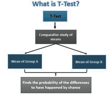
A t-test is a statistical method used to compare the means of two groups and determine if there is a significant difference between them. It is particularly useful when working with data that follows a normal distribution and has unknown variances, like the results obtained from flipping a coin multiple times.
Essentially, the t-test is a tool for hypothesis testing in statistics. It relies on the t-statistic, t-distribution values, and degrees of freedom to establish statistical significance.
Key Takeaways
- A t-test is employed to ascertain whether there is a notable difference between the means of two variables.
- It serves as a crucial method for hypothesis testing in statistics.
- When conducting a t-test, you need to consider three key data values: the disparity between the mean values of each dataset, the standard deviation of each group, and the number of data points.
- T-tests can be categorized as dependent or independent based on the nature of the data being analyzed.
Understanding the T-Test
- The t-test compares the average values of two data sets to determine whether they come from the same population. For example, if we compare a sample of students from class A with a sample from class B, their mean and standard deviation are unlikely to be identical. Similarly, samples from a placebo control group and a drug treatment group will likely have slightly different means and standard deviations.
- In practice, a t-test draws samples from two sets and sets up a problem statement with a null hypothesis, assuming the means of both groups are equal. After calculating the relevant values and comparing them to standard values, the null hypothesis is either accepted or rejected. Rejecting the null hypothesis suggests that the observed differences in data are statistically significant and not due to chance.
- The t-test is one of several statistical methods used for this purpose. Statisticians may choose other tests like the z-test for larger samples or the chi-square and f-tests to handle different variables or more complex analyses.
Using a T-Test
Consider a scenario where a pharmaceutical company conducts a test on a new medication. In this test, one group of patients is given the new drug, while another group, known as the control group, is given a placebo. A placebo is a substance without any therapeutic effects, used as a reference point to evaluate how the group receiving the actual drug reacts.
Following the trial, it is observed that the average increase in life expectancy for the control group, who received the placebo, is three years. On the other hand, the group that received the new medicine showed an average increase in life expectancy of four years.
While this initial observation suggests that the drug is effective, there is a possibility that these results could be due to random chance. To validate these findings and determine their applicability to the broader population, a statistical tool called a t-test is employed.
Assumptions for Using a T-Test:
- Data Nature: The collected data should be on a continuous or ordinal scale, like IQ test scores.
- Random Sampling: Data collection must stem from a randomly chosen segment of the overall population.
- Distribution: The data should yield a normal distribution resembling a bell-shaped curve.
- Variance Equality: There should be uniform or homogenous variance, indicating that standard deviations are equal.
T-Test Formula
The t-test calculation relies on three key data points: the mean difference between the two data sets, the standard deviation of each group, and the sample size of each group.
This analysis helps determine whether the difference between the groups is due to chance or represents a meaningful difference in the study. The t-test essentially assesses if the observed difference is statistically significant or simply a random variation.
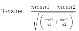
The t-test generates two main outputs: the t-value (or t-score) and the degrees of freedom. The t-value represents the ratio of the difference between the means of the two samples to the variability within the samples.
The numerator is the difference between the means of the two sample sets, while the denominator reflects the variation within the samples, which measures the dispersion or variability.
This calculated t-value is then compared to a critical value from the T-distribution table. A higher t-value indicates a larger difference between the two sample sets, while a smaller t-value suggests greater similarity between them.
T-Score
- A large t-score signifies significant differences between the groups.
- A small t-score indicates similarity between the groups.
Paired Sample T-Test
The paired sample t-test, also known as the correlated t-test, is a type of statistical test used when dealing with matched pairs of similar units or cases involving repeated measures. For instance, it is applicable when testing the same individuals before and after a treatment.
Application:
This test is suitable for scenarios where samples are related or possess similar characteristics. It is commonly used in studies involving comparisons within related groups like children, parents, or siblings.
Formula:
The formula for calculating the t-value and degrees of freedom in a paired t-test is:
Where:
- mean 1 and mean 2: The average values of the two sample sets.
- s(diff): The standard deviation of the differences between paired data values.
- n: The sample size (number of paired differences).
- n-1: The degrees of freedom.
Equal Variance or Pooled T-Test
The equal variance t-test, also known as the pooled t-test, is an independent t-test utilized when the sample sizes in each group are equal or when the variances of the two datasets are similar.
The formula used for calculating t-value and degrees of freedom for equal variance t-test is:
where:
mean 1 and mean 2: Average values of each sample set
var 1 and var 2: Variances of each sample set
n1 and n2: Number of records in each sample set
and,
Degrees of Freedom = n1 + n2 − 2
where:
n1 and n2 = Number of records in each sample set
Unequal Variance T-Test
Unequal Variance T-Test is a type of independent t-test utilized when the sample sizes and variances between two groups differ. This method is also known as Welch's t-test.
The formula used for calculating t-value and degrees of freedom for an unequal variance t-test is:

where:
mean1 and mean2 = Average values of each
of the sample sets
var1 and var2 = Variance of each of the sample sets
n1 and n2 = Number of records in each sample set
and,
where:
var1 and var2 = Variance of each of the sample sets
n1 and n2 = Number of records in each sample set
Which T-Test to Use?
The following flowchart helps in deciding which t-test to use based on the characteristics of the sample sets. Key considerations include how similar the sample records are, the number of data records in each sample set, and the variance of each sample set.
Example of an Unequal Variance T-Test
Imagine measuring the diagonal of paintings in an art gallery. One group has 10 paintings, while the other has 20. Let's look at the data sets with mean and variance values:

Though the mean of Set 2 is higher than that of Set 1, we cannot immediately conclude that the population corresponding to Set 2 has a higher mean than the population corresponding to Set 1.
To determine whether the difference between the means, from 19.4 to 21.6, is due to chance or reflects real differences between the overall populations of the paintings received by the art gallery, we establish a null hypothesis, which assumes the means are equal for both sample sets. A t-test is then conducted to evaluate the plausibility of this hypothesis.
Given that the sample sizes differ (n1 = 10 and n2 = 20) and their variances are unequal, the t-value and degrees of freedom are calculated according to the formula for an Unequal Variance T-Test.
The t-value calculated is -2.24787. Since the sign can be disregarded when comparing t-values, we use 2.24787 for the comparison.
The degrees of freedom, calculated as 24.38, are rounded down to 24 based on the formula requirements.
We set a significance level (alpha level or p-value) as the acceptance criterion, typically at 5%. For 24 degrees of freedom and a 5% significance level, the t-distribution table gives a critical value of 2.064. Since the calculated t-value of 2.247 is greater than the table value, we reject the null hypothesis that there is no difference between the means. This suggests that the population sets differ in a meaningful way, beyond chance alone.
How is the T-Distribution Table Used?
The T-Distribution Table comes in two formats: one-tail and two-tail. The one-tail format is used when there is a clear direction to be tested, such as assessing whether an output is less than or greater than a fixed value (e.g., determining the probability of getting a value below -3 or rolling more than seven on a pair of dice). The two-tail format is used for range-based analyses, such as testing whether a value falls between -2 and +2.
What is an Independent T-Test?
In an independent t-test, the samples are chosen independently of each other, meaning that the data in the two groups do not refer to the same subjects or values. For example, if 100 randomly selected patients are divided into two groups of 50, with one group serving as the control and receiving a placebo, and the other receiving a treatment, these two groups are independent, unpaired, and unrelated.
What Does a T-Test Explain and How Is It Used?
A t-test is a statistical method used to compare the means of two groups. It is frequently employed in hypothesis testing to determine whether a treatment or process has a significant effect on the population of interest, or whether two groups are statistically different from each other.
What is a Z-Test?

A z-test is a statistical method used to determine whether two population means differ when variances are known and sample sizes are large. It can also compare a sample mean to a hypothesized value. The data should approximate a normal distribution, and parameters such as variance and standard deviation must be calculated for a z-test to be performed.
Key Points:
- A z-test is used to assess whether two population means are different or to compare a sample mean to a hypothesized value when variances are known and the sample size is large.
- Z-tests apply to normally distributed data and use a z-statistic (or z-score) as the result.
- Z-tests are related to t-tests, but t-tests are more appropriate for small sample sizes and when the standard deviation is unknown.
- Z-tests assume the standard deviation is known, while t-tests assume it is not.
Understanding Z-Tests
A z-test is a hypothesis test in which the z-statistic follows a normal distribution. It is best used for samples larger than 30, as the central limit theorem indicates that larger sample sizes lead to approximately normal distributions.
When conducting a z-test, the null and alternative hypotheses must be stated, along with the alpha level. A z-score (test statistic) is calculated, and the results and conclusion are drawn. A z-score shows how many standard deviations a sample score is above or below the population mean.
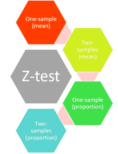
Z-tests can include one-sample location tests, two-sample location tests, paired difference tests, and maximum likelihood estimates. Z-tests are closely related to t-tests, which are better suited for small sample sizes when the standard deviation is unknown. If the standard deviation of the population is unknown, the sample variance may be used as an approximation.
Z-Score Formula:
The z-score is calculated using the formula:

Where:
- z is the z-score
- x is the value being evaluated
- μ is the population mean
- σ is the population standard deviation
One-Sample Z-Test Example
An investor wants to determine if the average daily return of a stock exceeds 3%. A random sample of 50 returns is taken, showing an average return of 2%. Assuming a standard deviation of 2.5%, the null hypothesis states that the mean return is 3%.
The alternative hypothesis tests whether the mean return differs from 3%. An alpha level of 0.05 is chosen for a two-tailed test, placing 0.025 in each tail. The critical values are ±1.96. If the calculated z-value exceeds 1.96 or is below -1.96, the null hypothesis is rejected.
To calculate the z-value, subtract the hypothesized mean of 3% from the observed sample mean of 2%, then divide the result by the standard deviation divided by the square root of the sample size. This gives:

Since -2.83 is less than -1.96, the null hypothesis is rejected, leading to the conclusion that the average daily return is less than 3%.
Difference Between a Z-Test and a T-Test
Z-tests are similar to t-tests, but t-tests are more appropriate for small sample sizes (fewer than 30). Z-tests assume that the population standard deviation is known, whereas t-tests assume it is unknown.
When to Use a Z-Test
A z-test is used when the population standard deviation is known and the sample size is at least 30. If the population standard deviation is unknown, regardless of sample size, a t-test is used instead.
What is a Z-Score?
A z-score, or z-statistic, measures how many standard deviations a data point is from the population mean. A z-score of 0 means the data point equals the mean, while a z-score of 1.0 means it is one standard deviation above the mean. Positive z-scores indicate values above the mean, while negative z-scores indicate values below it.
Central Limit Theorem (CLT)
The central limit theorem (CLT) states that the distribution of sample means approaches a normal distribution as sample size increases, regardless of the population's shape, provided all samples are identical in size. For most practical purposes, a sample size of 30 or more is sufficient for the CLT to hold, which justifies using the z-test.
Z-Test Assumptions
To perform a z-test, the population must be normally distributed, the samples must have equal variance, and the data points should be independent of each other.
Conclusion
A z-test is a tool for hypothesis testing to determine whether a relationship or result is statistically significant. It is used to test whether two means are equal (the null hypothesis) and can only be applied when the population standard deviation is known and the sample size is 30 or more. Otherwise, a t-test should be used.
|
157 videos|236 docs|166 tests
|
FAQs on Hypothesis Testing: t-test & z-test - Crash Course for UGC NET Commerce
| 1. What is a T-Test? |  |
| 2. When should I use a T-Test? |  |
| 3. What is the difference between a T-Test and a Z-Test? |  |
| 4. How do I interpret the results of a T-Test? |  |
| 5. What is a Z-Score and how is it related to Z-Tests? |  |


