Riemann Integration (Definite Integrals and their Properties) | Mathematics Optional Notes for UPSC PDF Download
| Table of contents |
|
| What is Riemann Integral? |
|
| Riemann Sums |
|
| Riemann Integral Formula |
|
| Properties of Riemann Integral |
|
| Applications of Riemann Integral |
|

What is Riemann Integral?
Riemann integral is a method in calculus to find the total area under a curve between two points. It involves dividing the area into small rectangles and adding up their areas to approximate the total area under the curve. As the width of these rectangles approaches zero, the sum of their areas gives the exact value of the integral.
Riemann Integral Definition
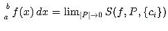
- The function (f) is Riemann integrable on [a, b] if the limit of the Riemann sums exists as the norm of the partition approaches zero, independently of the choice of sample points ci.
- This limit is called the Riemann integral of f over [a, b] and is denoted by:
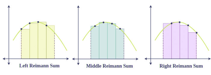
Riemann Sums
- Riemann sums are a way to estimate the total area under a curve by breaking it into smaller pieces. Imagine dividing the area under the curve into rectangles. By adding up the areas of these rectangles, we get an approximation of the total area under the curve.
- The more rectangles we use, the closer our estimate gets to the actual area. Riemann sums help us understand and calculate the total accumulation or value represented by a curve within a specific interval.
- For Example: To find the area under the curve y = x2 between x = 0 and x = 2.
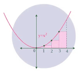
- We can use Riemann sums to approximate this area by dividing the interval [0, 2] into smaller subintervals and approximating the area of each subinterval with a rectangle.
- Let's say we divide the interval into four equal subintervals: [0, 0.5], [0.5, 1], [1, 1.5] and [1.5, 2].
- For each subinterval, we find the height of the rectangle by evaluating the function y=x2 at a specific point within the subinterval. For simplicity, let's choose the left endpoint of each subinterval.
For the first subinterval [0, 0.5], the height of the rectangle is y = (0)2 = 0.
For the second subinterval [0.5, 1], the height of the rectangle is y = (0.5)2 = 0.25.
For the third subinterval [1, 1.5], the height of the rectangle is y = (1)2 = 1.
For the fourth subinterval [1.5, 2], the height of the rectangle is y = (1.5)2= 2.25.
Multiply each height by the width of the corresponding subinterval (which is 0.50.5 in this case) to find the area of each rectangle.
Now add up the areas of all the rectangles to get an approximation of the total area under the curve.
In this example, the sum of the areas of the rectangles is approximately 0×0.5 + 0.25×0.5 + 1×0.5 + 2.25×0.5 = 1.125
So, the Riemann sum approximation of the area under the curve y=x2 between x=0 and x=2 is approximately 1.125 square units.
Riemann Integral Formula
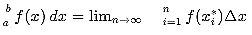
- Riemann integral formula represents the calculation of the integral of a function over a specified interval. In its basic form, for a function f(x) defined on the interval [a,b], the Riemann integral is given by:

- This notation represents the sum of infinitely many infinitely small rectangles under the curve of the function f(x) between x = a and x=b.
- The integral symbol ∫∫ represents integration, f(x) is the function being integrated, dx denotes the variable of integration, and a and b are the lower and upper limits of integration, respectively.
Properties of Riemann Integral
Riemann integral possesses several important properties that make it useful in calculus and analysis. Here are some key properties:
1. Linearity
The Riemann integral is linear, meaning that it satisfies the properties of additivity and scalar multiplication. That is, for functions f(x) and g(x) and constants c and d, we have:
2. Additivity
The integral of a sum of functions is the sum of their integrals. That is, for functions f(x) and g(x), we have: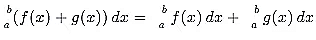
3. Monotonicity
Monotonicity property of the Riemann integral sates that if one function is always greater than or equal to another function over an interval, then the integral of the first function should be greater than or equal to the integral of the second function over that interval. Let f and g be two Riemann integrable functions on the closed interval [a, b]. If f(x) ≤ g(x) for all x ∈ [a, b], then: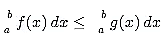
4. Constant Multiple Rule
The integral of a constant multiple of a function is the constant multiplied by the integral of the function. That is, for a constant c, we have:
5. Interval Splitting
The integral over a sum of intervals is the sum of the integrals over each individual interval. That is, for intervals [a,c] and [c,b], we have:
6. Order Preservation
If f(x) is non-negative on an interval [a,b] and f(x) ≥ g(x) for all x in [a,b], then: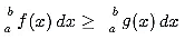
Applications of Riemann Integral
The Riemann integral finds application across various fields:
- Integration and Differential Calculus: It's fundamental in calculus for finding areas under curves and solving problems related to rates of change, such as velocity and acceleration.
- Physics Problems: Used extensively in physics for calculating quantities like work, energy, and fluid flow rates. It helps in analyzing continuous phenomena and predicting outcomes.
- Partial Differential Equations: Applied in solving partial differential equations, which describe how functions change in response to changes in multiple variables. This is crucial in fields like engineering and physics.
- Trigonometric Series: Utilized in representing functions as trigonometric series, which can simplify complex functions into a sum of simpler trigonometric functions.
- Measurement of Distance Traveled: In scenarios where an object's velocity changes over time, the Riemann integral can determine the total distance traveled by analyzing the area under the velocity-time graph. This concept helps in understanding motion and predicting trajectories accurately.
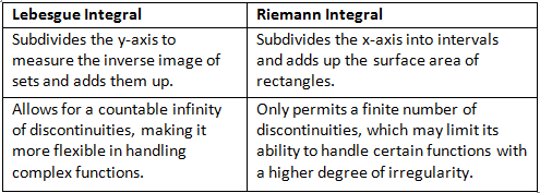
Difference Between Lebesgue Integral and Riemann Integral
The difference between Lebesgue integral and Riemann integral can be understood from the table below:
Examples of Riemann Integral
Example 1: Compute Riemann integral of function f(x) = x3 over the interval [−2, 2].
Sol:
Riemann integral of f(x) over [a,b] is given by:
where Δx = nb−a is the width of each subinterval, and xi∗ is any point in the ith subinterval.
In this case, a = −2, b = 2, and f(x) = x3.
First, we need to partition the interval [−2,2] into n equal subintervals. Let's choose n=4 for simplicity.
Δx=[2−(−2)]/4=4/4=1
So, the subintervals are [−2,−1], [−1,0], [0,1], and [1,2].
Next, we'll choose a point in each subinterval to evaluate f(x). Let's choose the midpoint of each subinterval:
- For [−2,−1]: x1∗= −1.5
- For [−1,0]: x2∗= −0.5
- For [0,1]: x3∗= 0.5
- For [1,2]: x4∗= 1.5
Now, we'll evaluate f(x)=x3 at each point:
- f(−1.5) = (−1.5)3 = −3.375
- f(−0.5) = (−0.5)3 = −0.125
- f(0.5) = (0.5)3 = 0.125
- f(1.5) = (1.5)3 = 3.375
Finally, we'll sum up the products of
and Δx for each subinterval and take the limit as n approaches infinity.
[(−3.375)(1)+(−0.125)(1)+(0.125)(1)+(3.375)(1)]
=limn→∞(−3.375−0.125+0.125+3.375)
=limn→∞0 = 0
Therefore, the Riemann integral of f(x) = x3 over the interval [−2,2] is 0.
Example 2: Find Riemann integral of function f(x) = ex over the interval [0, 2].
Sol:
Riemann integral of f(x) over [a,b] is given by:
where Δx=nb−a is the width of each subinterval, and xi∗ is any point in the ith subinterval.
In this case, a=0, b=2, and f(x)=ex.
First, we need to partition the interval [0,2] into n equal subintervals. Let's choose n=4 for simplicity.
So, the subintervals are [0,0.5], [0.5,1], [1,1.5], and [1.5,2].
Next, we'll choose a point in each subinterval to evaluate f(x). Let's choose the right endpoint of each subinterval:
- For [0,0.5]: x1∗ = 0.5
- For [0.5,1]: x2∗ = 1
- For [1,1.5]: x3∗ = 1.5
- For [1.5,2]: x4∗ = 2
Now, we'll evaluate f(x)=ex at each point:
- f(0.5) = e0.5
- f(1) = e1
- f(1.5) = e1.5
- f(2) = e2
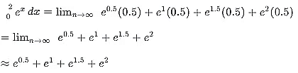
Finally, we'll sum up the products of f(xi∗) and Δx for each subinterval and take the limit as n approaches infinity.
Thus, Riemann integral of f(x)=ex over the interval [0,2] is approximately e0.5+e1+e1.5+e2.
|
397 videos|311 docs
|
FAQs on Riemann Integration (Definite Integrals and their Properties) - Mathematics Optional Notes for UPSC
| 1. What is the Riemann Integral and how is it defined? |  |
| 2. What are Riemann Sums and how do they relate to the Riemann Integral? | |
| 3. What are some key properties of the Riemann Integral? | |
| 4. How does the Riemann Integral differ from the Lebesgue Integral? | |
| 5. Can you provide an example of calculating a Riemann Integral? | |


ppt
,MCQs
,Previous Year Questions with Solutions
,Riemann Integration (Definite Integrals and their Properties) | Mathematics Optional Notes for UPSC
,Summary
,Riemann Integration (Definite Integrals and their Properties) | Mathematics Optional Notes for UPSC
,Free
,Exam
,video lectures
,Important questions
,Objective type Questions
,study material
,mock tests for examination
,Extra Questions
,Semester Notes
,practice quizzes
,Viva Questions
,Sample Paper
,past year papers
,shortcuts and tricks
,Riemann Integration (Definite Integrals and their Properties) | Mathematics Optional Notes for UPSC
;


Riemann Integration (Definite Integrals and their Properties) Free PDF Download
Importance of Riemann Integration (Definite Integrals and their Properties)
Riemann Integration (Definite Integrals and their Properties) Notes
Riemann Integration (Definite Integrals and their Properties) UPSC Questions
Study Riemann Integration (Definite Integrals and their Properties) on the App
|
© EduRev
|
Education Revolution
|


|


