Determination of Income and Employment Class 12 Economics
Introduction
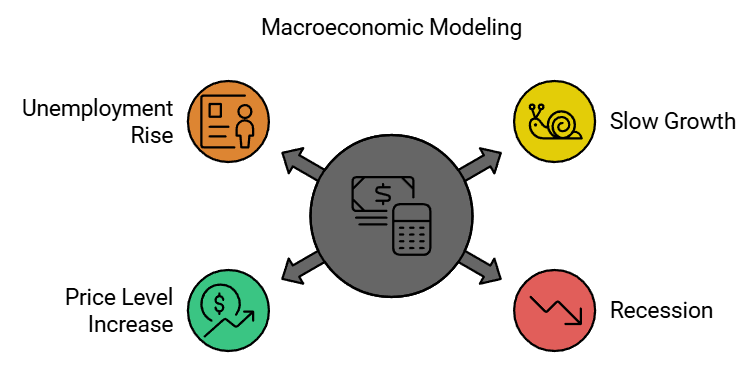
- The main aim of macroeconomics is to create theoretical tools, known as models, which can explain the processes that determine the values of certain variables.
- These models seek to answer important questions, such as what leads to periods of slow growth or recession in the economy, increases in the price level, or rises in unemployment.
- It is challenging to consider all variables at once. Therefore, when focusing on a specific variable, we keep the values of all other variables unchanged.
- This approach is known as the assumption of ceteris paribus, which means "other things being equal."
- To understand the relationship between two variables, say x and y, we first solve one equation for x in terms of y, and then substitute this back into another equation to find the complete solution.
- We use the same method when analyzing the macroeconomic system.
- This chapter focuses on determining National Income while assuming that the prices of final goods and the interest rate remain constant.
- The theoretical model discussed in this chapter is based on the ideas of John Maynard Keynes.
Aggregate Demand and Its Components
- In the chapter about National Income Accounting, we come across terms like consumption, investment, and the total output of final goods and services in an economy, known as GDP.
- These terms can have two meanings. In Chapter 2, they were used in an accounting sense, which refers to the actual values of these items as measured by what happens in the economy in a specific year. We call these actual values ex-post measures.
- However, these terms can also be understood differently. For example, consumption might refer not to what people actually consumed in a year, but to what they planned to consume during that time.
- Similarly, investment can refer to how much a producer intends to add to her inventory, which might differ from what she actually does.
- For instance, if a producer plans to increase her stock by Rs 100 by the end of the year, her planned investment would be Rs 100.
- If there is an unexpected rise in demand for her products, and she sells more than she expected, she may need to reduce her planned inventory.
- Suppose she sells Rs 30 worth of goods more than she planned. This means that by the end of the year, her inventory only increases by Rs (100 - 30) = Rs 70.
- Thus, her planned investment is Rs 100, but her actual investment, or ex-post investment, is only Rs 70.
- We refer to the planned values of items like consumption, investment, or output as ex-ante measures.
- In simpler terms, ex-ante reflects what has been planned, while ex-post reflects what has happened.
- To understand how income is determined, it is important to know the planned values of the different parts of aggregate demand.
- Next, we will examine these components in more detail.
Consumption
- The demand for goods and services that are utilized by individuals for day-to-day consumption in an economy is referred to as consumption.
- Household income plays a crucial role in determining consumption. Generally, an increase in income results in an increase in consumption expenditure, while a decrease in income leads to a decrease in consumption.
- A consumption function is used to describe the relationship between consumption and income. The simplest form of a consumption function assumes that consumption changes at a constant rate in response to changes in income.
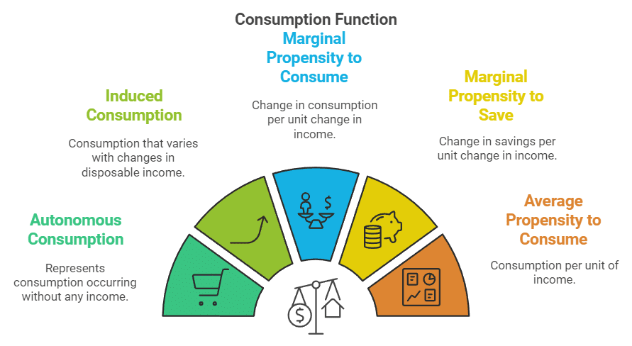
Several significant terms are associated with the Consumption Function:
Autonomous and Induced Consumption
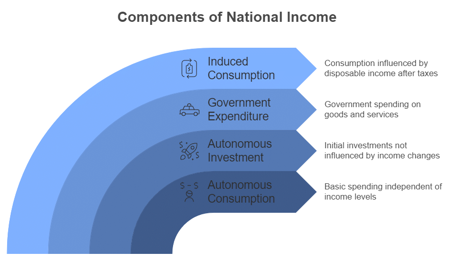
- This represents a certain level of consumption that takes place even when income is zero. This level of consumption is independent of income and is thus referred to as autonomous consumption.

- The equation mentioned is known as the consumption function.
- In this function, C represents the consumptionexpenditureby households. This expenditure includes two parts:
- Autonomous consumption, which is shown by
 , refers to the level of consumption that occurs regardless of income.
 - Induced consumption, represented as cY, indicates how consumption is affected by income.
- Autonomous consumption, which is shown by
- Autonomous consumption is important because it means that consumption can still happen even if income is zero.
- The induced component of consumption, cY, highlights the connection between consumption and income levels.
- The induced component of consumption, represented as cY, shows how consumption depends on income.
- When income increases by Re 1, the induced consumption also increases by the marginal propensity to consume (MPC), which is denoted as c.
- This relationship can be understood as the rate at which consumption changes when income changes.
Marginal Propensity to Consume (MPC)
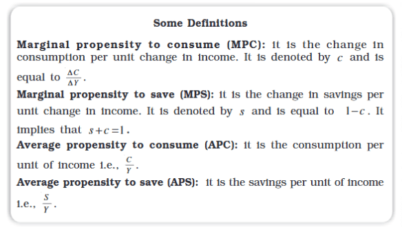
- This refers to the change in consumption per unit change in income. The MPC ranges between 0 and 1, which means that either the consumer does not increase consumption at all (MPC = 0) or uses the entire change in income on consumption (MPC = 1) or uses part of the change in income for changing consumption (0 < MPC < 1).

- For example, the country Imagenia has a consumption function represented by the equation C = 100 + 0.8Y.
- This equation shows that even when the people of Imagenia have no income, they still consume goods worth Rs. 100.
- The term autonomous consumption refers to the 100 in the equation, which is the base level of consumption regardless of income.
- Imagenia's marginal propensity to consume (MPC) is 0.8.
- This means that for every increase of Rs. 100 in income, the consumption will rise by Rs. 80.
- In summary, higher income leads to greater consumption, specifically 80% of any income increase.
Marginal Propensity to Save (MPS)
- Now, let's consider savings. Savings is the part of income that is not spent on consumption.
- We can express this with the formula:
S = Y - C
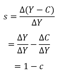
where S is savings, Y is income, and C is consumption. - The marginal propensity to save (MPS) indicates how much savings change when income increases.

Since S = Y - C
Investment
- Investment is defined as an addition to the stock of physical capital (such as machines, buildings, roads etc., i.e. anything that adds to the future productive capacity of the economy) and changes in the inventory (or the stock of finished goods) of a producer.
- Note that ‘investment goods’ (such as machines) are also part of the final goods – they are not intermediate goods like raw materials.
- Machines produced in an economy in a given year are not ‘used up’ to produce other goods but yield their services over a number of years.
- Investment decisions by producers, such as whether to buy a new machine, depend, to a large extent, on the market rate of interest.
- However, for simplicity, we assume here that firms plan to invest the same amount every year.
- We can write the ex-ante investment demand as:

where is a positive constant that represents the autonomous (given or exogenous) investment in the economy in a given year.
Determination of Income in a Two-Sector Model
- In a situation where there is no government, the total expected demand for final goods is calculated by adding together the expected spending by consumers and the expected spending on investments.
- This relationship can be expressed as: AD = C + I.
- In this formula:
- AD stands for Aggregate Demand.
- C represents Consumption Expenditure, which is the amount that households plan to spend on goods and services.
- I denotes Investment Expenditure, which is the spending that businesses plan to make on capital goods.
- By substituting the values for C and Iusing the equations above, we can find the overall expected demand in the economy:

- If the final goodsmarketis in equilibrium this can be written as

where Y is the ex-ante, or planned, output of final goods. This equation can be further simplified by adding up the two autonomous terms:
where 
- In reality, the two parts of autonomous spending behave differently. C, which stands for the basic consumption level in an economy, tends to stay relatively stable over time.
- On the other hand, I has been seen to go through regular ups and downs.
Understanding the Equilibrium Equation
- It's important to be cautious when interpreting the term Y on the left side of the equilibrium equation. This Y represents the planned output or the intended supply of final goods.
- Meanwhile, the expression on the right side indicates the planned total demand for final goods in the economy.
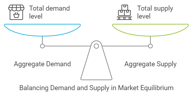
- The planned supply equals the planned demand only if the final goods market is balanced, meaning the economy is in equilibrium.
- If the planned demand for final goods is less than what producers plan to make in a certain year, the equilibrium equation will not hold true.
- This situation leads to an accumulation of inventory in warehouses, which we can view as an unintended buildup of stocks.
- It's important to understand that inventories refer to the portion of goods produced that has not been sold and remains with the company. Change in inventory is referred to as inventory investment.
- Inventory investment can be either negative or positive:
1. If there is an increase in inventory, this is considered positive inventory investment.
2. If inventory decreases, it is seen as negative inventory investment. - Inventory investment can happen for two main reasons:
1. The company decides to keep some stock for various reasons, which is called planned inventory investment.
2. Sales may differ from what was expected, leading the company to either increase or reduce existing inventory, known as unplanned inventory investment. - Therefore, even if the planned Y is greater than the planned C + I, the actual Y will equal the actual C + I, with any extra output resulting in unintended inventory accumulation in the actual I on the right side of the accounting identity.
Government's Role
- Now, let's introduce the government into this economy. The main economic actions of the government that influence the total demand for final goods and services can be summarized by two fiscal variables: Tax (T) and Government Expenditure (G), both of which are considered independent in our analysis.
- The government, through its spending G on final goods and services, contributes to the overall demand just like other businesses and households.
- Taxes set by the government take away a portion of a household's income. This means that the disposable income becomes: Yd = Y - T
- Households only use a part of this disposable income for spending. Therefore, we need to change equation (4.3) to include the government's role: Y = C + I + G + c(Y - T)
- Here, G - c.T is similar to C or I, and it simply adds to the overall term A. This change does not really affect the overall analysis in any major way.
- For simplicity, we will ignore the government sector for the rest of this chapter.
- It's important to note that without the government putting taxes and subsidies in place, the total value of goods and services produced in the economy, known as GDP, becomes equal to National Income.
- From now on, we will refer to Y as either GDP or National Income interchangeably throughout the rest of this chapter.
Determination of Equilibrium Income in the Short Run
- In microeconomic theory, when we look at the balance of demand and supply in a single market, both the demand and supply curves help us find the equilibrium price and equilibrium quantity at the same time.
- In macroeconomic theory, we follow a two-step process:
1. First, we determine the macroeconomic equilibrium by keeping the price level constant.
2. Second, we allow the price level to change and then analyze the macroeconomic equilibrium again. - Why do we assume the price levelis fixed in the first step? There are two reasons:
1. First, we assume there are unused resources in the economy, such as machines, buildings, and labour. In this case, the law of diminishing returns does not apply, meaning we can produce more output without raising the marginal cost. Therefore, the price level stays the same, even if the amount produced changes.
2. Second, this is a simplifying assumption that we will adjust later on.
Macroeconomic Equilibrium with Price Level Fixed
A. Graphical Method
- As already explained, the consumer's demand can be expressed by the equation:

- This can be shown on a graph with the help of a linear equation:
Y = a + bX - Here, the variables X and Y have a linear relationship between them.
- The constants a and b are part of this equation.
- This equation is shown in as below:
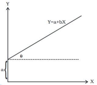
- The constant a represents the intercept on the Y-axis. This means it is the value of Y when X is zero.
- The constant b indicates the slope of the line. In other words, it is the ratio of the rise over the run, represented by the tangent of the angle θ, where tan θ = b.
Consumption Function: Graphical Representation
Using the same logic, the consumption function can be shown as follows:
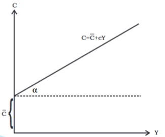
Consumption function, where: = intercept of the consumption function
c = slope of consumption function = tan α
Investment Function: Graphical Representation
- In a two-sector model, there are two main sources of final demand: consumption and investment
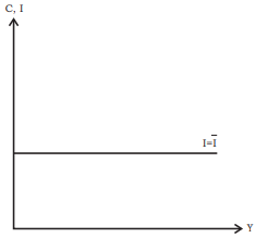
- The investment function is represented as

- On a graph, this is depicted as a horizontal line positioned at a height equal to I above the horizontal axis.
- In this model, I is considered autonomous, meaning it remains constant regardless of the level of income.
Aggregate Demand: Graphical Representation
- The Aggregate Demand function illustrates the overall demand, which includes consumption and investment, at various income levels.
- In graphical terms, the aggregate demand function can be created by adding together the consumption and investment functions vertically.
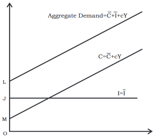
- The aggregate demand function is similar to the consumption function, meaning they have the same slope, which is c.
- This function represents ex-ante demand, indicating what people plan to buy in the future.
Supply Side of Macroeconomic Equilibrium
- In microeconomic theory, the supply curve is illustrated on a graph with price on the vertical axis and quantity supplied on the horizontal axis.
- In the initial stage of macroeconomic theory, we consider the price level to be constant.
- Here, aggregate supply or GDP is thought to change smoothly, as there are unused resources of all kinds available.
- Regardless of the GDP level, that amount will be supplied, and the price level does not affect it.
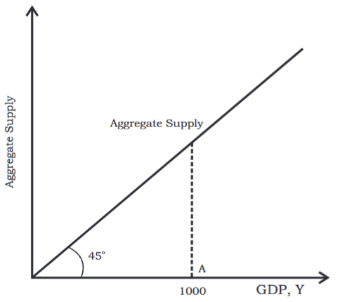
- This situation of supply is represented by a 45-degree line.
- The 45-degree line has the characteristic that each point on it has the same horizontal and vertical coordinates.
- For example, if the GDP is Rs.1,000 at point A, then the amount supplied will be Rs.1,000 worth of goods.
- To show this point, the supply at point A corresponds to point B, which is found at the intersection of the 45-degree line and the vertical line at A.
Equilibrium
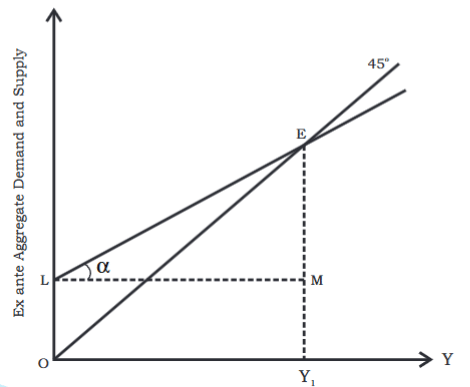
- Equilibrium is represented visually by combining ex-ante aggregate demand and supply in the diagram below.
- The point at which ex-ante aggregate demand matches ex-ante aggregate supply indicates equilibrium.
- Therefore, the equilibrium point is marked as E.
- The equilibrium level of income is shown as OY1.
B. Algebraic Method
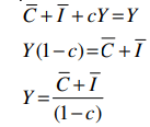
Ex-ante aggregate demand (Y): 
- Equilibrium happens when the plans of suppliers align with the plans of those who create the final demand in the economy.
- In this context, it is important that the total planned demand equals the total planned supply before any transactions occur.
- This means that ex-ante (or before the fact) aggregate demand must equal ex-ante aggregate supply.
Effect of an Autonomous Change in Aggregate Demand on Income and Output
- The level of income at equilibrium relies on aggregate demand.
- When aggregate demand changes, the equilibrium income level also changes.
- This change can occur due to:
- Change in consumption(autonomous or induced)
- Change in investment: Investment is considered autonomous, meaning it does not depend on income. However, several factors can influence investment, including:
- Availability of credit: When credit is easy to get, investment tends to increase.
- Interest rates: Higher interest rates increase the cost of borrowing, causing firms to reduce their investment.
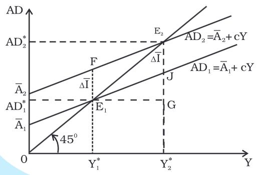
- To illustrate changes in investment, consider the following example:
- Let C equal 400 and I equal 10. The equilibrium income calculated from the equation Y = AD is 250.
- If investment rises to 20, the new equilibrium income increases to 300.
- This increase can be visualized in a graph.
- The rise in income reflects the increase in investment, which is part of autonomous expenditure.
- When autonomous investment goes up, the AD1 line shifts upward to a new position AD2.
- At the output level Y*, the value of aggregate demand becomes Y*F, which is greater than the previous output 0Y*.
- The amount E1F indicates the excess demand created by the increase in autonomous expenditure.
- As a result, E1 no longer indicates the equilibrium.
- To find the new equilibrium in the goods market, we look for where the new aggregate demand line AD2 meets the 45-degree line.
- This intersection occurs at point E2, which is now the new equilibrium point.
- In this new equilibrium, both output and aggregate demand have increased by an amount equal to E1G = E2G, which is more than the initial increase in autonomous expenditure, represented as ΔI = E1F = E2J.
- This suggests that the initial rise in autonomous expenditure has a multiplier effect on the equilibrium values of aggregate demand and output.
- The next section will discuss why aggregate demand and output can increase by a larger amount than the initial rise in autonomous expenditure.
The Multiplier Mechanism
- In the previous section, we saw that if there is an increase in autonomous expenditure by 10 units, the resulting change in equilibrium income is 50 units, moving from 250 to 300.
- This can be understood through the multiplier mechanism, which works as follows:
- The production of final goods requires factors of production such as labour, capital, land, and entrepreneurship.
- Without indirect taxes or subsidies, the total value of final goods produced is shared among different factors:
- wages are paid to labour,
- interest goes to capital,
- rent is paid for the land,
- The remaining amount is kept by the entrepreneur as profit.
- The total of these payments in the economy is known as National Income, which equals the total value of final goods produced, or GDP.
- In our example, the additional output of 10 units is distributed among various factors, leading to a rise in the economy's income by 10.
- As income rises by 10, consumption expenditure increases by (0.8) * 10, because people spend 0.8 (the marginal propensity to consume or mpc) of their extra income on consumption.
- This results in a new total demand in the economy that goes up by (0.8) * 10, creating excess demand of the same amount.
- In the next production cycle, producers will increase their planned output by (0.8) * 10 to meet this excess demand.
- When this additional output is shared among the factors, the economy's income increases by (0.8) * 10, and consumption demand rises further by (0.8) * 210, again generating excess demand.
- This process repeats itself in successive rounds:
- Producers keep increasing output to satisfy the excess demand,
- Consumers spend part of their new income on consumption, leading to even more excess demand in the next round.
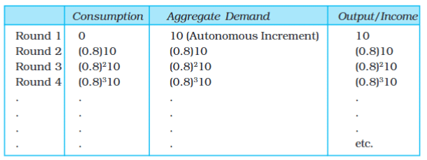
- To track the changes in aggregate demand and output in each round, we can refer to Table 4.1.
- The final column in the table shows the increases in the value of final goods output (and thus the economy's income) for each round.
- The second and third columns reflect the increases in total consumption expenditure and aggregate demand respectively.
- To calculate the total increase in output of final goods, we can add up the infinite geometric series in the last column:
10 + (0.8) * 10 + (0.8)2 * 10 + ... = 10 {1 + (0.8) + (0.8)2 + ...} - This series sums up to:
10 / (1 - 0.8) = 50.
- The increase in the equilibrium value of total output is larger than the initial rise in autonomous spending.
- The ratio of the total increase in the equilibrium value of final goods output to the initial increase in autonomous spending is known as the investment multiplier of the economy.
- Remember that 10 and 0.8 represent the values of ΔI = ΔA and mpc, respectively.
- The formula for the multiplier can be understood as follows:

Paradox of Thrift
- If everyone in the economy decides to save a larger share of their income (meaning the marginal propensity to save or mps increases), the total amount of savings might not go up. Instead, it could either stay the same or even go down.
- This idea is referred to as the Paradox of Thrift. It suggests that when people try to be more careful with their money, they might end up saving less or the same amount as before.
- This concept may seem surprising, but it can be easily understood with the economic model we have studied.
- Let’s use an example to explain this. Imagine that at the starting point, the economy's income is at Y = 250. Suddenly, there is a change in how people spend their money—they become more cautious. This could happen because of news about a possible war or another serious situation, leading people to spend less.
- As a result, the mps increases, or the marginal propensity to consume (mpc) drops from 0.8 to 0.5. At the initial income level of AD1 = Y1 = 250, this drop in mpc means there will be a decrease in overall spending by an amount of (0.8 - 0.5) x 250 = 75.
- This reduction in spending can be seen as a sudden cut in consumption, which is caused by outside factors, not by changes within the model's variables.
- When overall demand decreases by 75, it becomes less than the output level of Y1 = 250. This creates a surplus of goods worth 75 in the economy.
- As a result, products start to pile up, and businesses decide to reduce their production by 75 in the next period to balance the market.
- However, this reduction in production leads to lower payments to workers, which means that people's income will drop by 75.
- With lower income, consumption also decreases, but this time it is based on the new mpc of 0.5. This means that spending will go down by (0.5) x 75, causing another surplus in the market.
- In the next round, producers will cut their output again by (0.5) x 75. Consequently, people's income will fall again, and spending will decrease by (0.5) x 2 x 75.
- This cycle continues, with each round resulting in smaller and smaller decreases in output and demand.
- However, as we can see from the decreasing amounts in each step, this process is moving towards a stable point.
- The important question is: what is the total reduction in the value of output and aggregate demand?
- To find the sum of the infinite series: 75 + (0.5) 75 + (0.5)2 75+ ... and so on to infinity.
- The total reduction in output is calculated as: 75 / (1 - 0.5) = 150
- This means the new equilibrium output of the economy is: Y*2 = 100
- People are now saving: S*2 = Y*2 - C*2
- = Y*2 - (C + c2Y*2)
- = 100 - (40 + 0.5 × 100) = 10 in total
- In the previous equilibrium, savings were: S*1 = Y*1 - C*1
- = Y*1 - (C + c1Y*1)
- = 250 - (40 + 0.8 × 250) = 10 at the previous marginal propensity to consume, c*1 = 0.8
- Thus, the total value of savings in the economy has stayed the same.
- When A changes, the line shifts up or down in parallel.
- When c changes, the line moves up or down. An increase in the marginal propensity to save (MPS) or a decrease in the marginal propensity to consume (mpc) lowers the slope of the aggregate demand (AD) line, causing it to tilt downwards.
- The situation is illustrated in the figure:
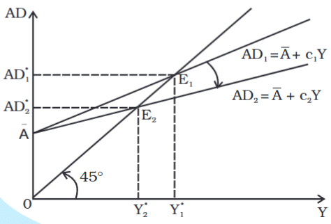
- With the initial values of the parameters: A = 50 and c = 0.8, the equilibrium value of the output and aggregate demand from equation (4.4) was: Y*1 = 50 / (1 - 0.8) = 250
- With the new value of the parameter c = 0.5, the new equilibrium value of output and aggregate demand is: Y*2 = 50 / (1 - 0.5) = 100
- The equilibrium output and aggregate demand have decreased by 150.
- As mentioned earlier, this means that the total value of savings has not changed.
Some More Concepts
- The level of output in the economy affects the amount of employment available, depending on the quantities of other production factors. This concept can be understood by looking at a production function on a large scale.
- When we say the output level is equal to aggregate demand (AD), it does not automatically mean everyone is employed.
- A full employment level of income is when all resources are used completely in the production process.
- Just because there is an equilibrium at the point where output equals demand does not mean that all resources are fully employed.
- Equilibrium means that if there are no changes, the income level in the economy will stay the same, even if there is some unemployment.
- The equilibrium output can be either higher or lower than the full employment output level.
- If the equilibrium output is lower than the full employment output, it means there is not enough demand to utilize all production factors. This situation is termed deficient demand, and it can lead to a decrease in prices over time.
- If the equilibrium output is higher than the full employment output, it indicates that the demand exceeds what can be produced at full employment. This situation is referred to as excess demand, and it can cause an increase in prices in the long run.
|
64 videos|308 docs|51 tests
|
FAQs on Determination of Income and Employment Class 12 Economics
| 1. What is aggregate demand and what are its main components? |  |
| 2. How does consumption influence aggregate demand? |  |
| 3. What role does investment play in the determination of income? |  |
| 4. How is equilibrium income determined in a two-sector model? |  |
| 5. What is the multiplier mechanism and how does it affect income and employment? |  |


